Table of Contents
A time series database is a database designed to store and analyze measurements or events indexed by time. It supports workloads such as sensor monitoring, application telemetry, and financial market analysis, where data arrives continuously and queries examine changes over time. InfluxDB 3 supports this model with timestamped data, SQL and InfluxQL queries, and line protocol ingestion.
What is time series?
Time series are simply measurements or events that are tracked, monitored, downsampled, and aggregated over time. Examples include average daily temperature, IIoT metrics, network telemetry, satellite instrumentation, website clicks, and financial market ticks.
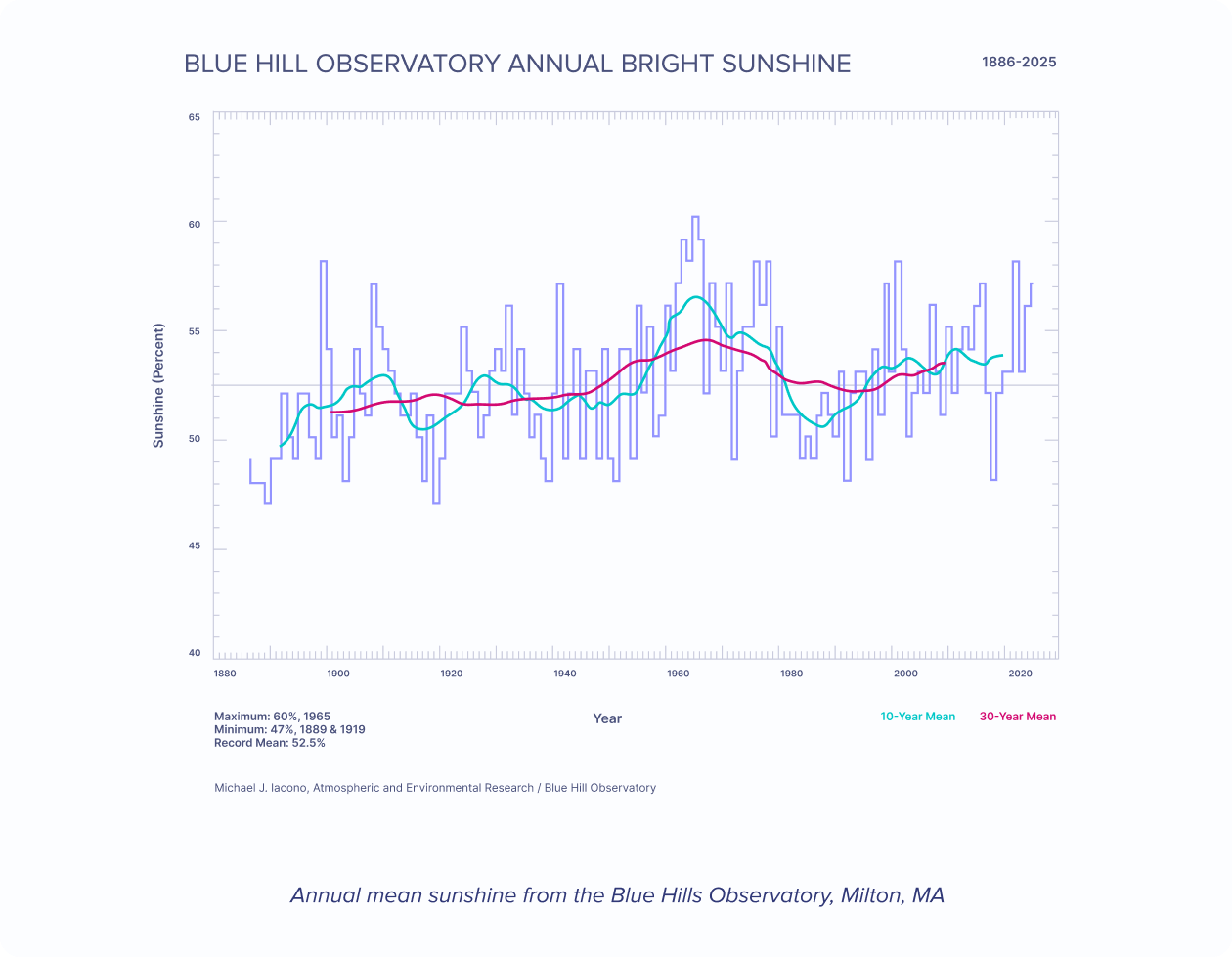
The defining feature of time series data is that it captures how a measurement changes over time. A simple way to determine if you’re working with a time series dataset, is to determine if one of your axes is time. Below are a few examples of time series data plotted on graphs:

Time series data appears in two forms: regular and irregular.
- Regular time series consist of measurements collected at regular intervals (every 10 seconds, for example). These are commonly referred to as metrics.
- Irregular time series consist of events generated by users, systems, or external stimuli, such as website clicks, financial market ticks, or application requests. These events occur whenever something happens, not on a fixed schedule.
Irregular time series are often transformed into regular representations through time-based aggregation. For example, individual request events can be summarized into one-minute average response times, or financial ticks can be aggregated into ten-minute average prices. The underlying data remains event-driven, but the analytical view becomes regular.
InfluxDB 3 can store both regularly sampled measurements and irregular timestamped events. The choice of database depends on the data model, query requirements, retention period, and surrounding tools; the comparison below explains these differences for several time series systems.
InfluxDB 3 organizes each point using a measurement (table) name, tags for metadata, fields for measured values, and a timestamp. Fields support floating-point numbers, signed and unsigned 64-bit integers, booleans, and strings. Queries select tables and filter or aggregate their time, tag, and field columns. See the line protocol reference for the write format.

This structure keeps an observation and its identifying metadata together. For example, a temperature reading can include a sensor ID and site as tags, a numeric temperature field, and the time it was measured.
What are the three time series workload patterns?
Time series workloads can be grouped into three overlapping patterns: operational monitoring, historical analysis, and digital engineering. Operational workloads respond to current conditions; analytical workloads explain past behavior; digital engineering workloads use those insights to inform models and automation.
| Workload pattern | Purpose | Typical query behavior | Example |
|---|---|---|---|
| Operational | Observe current conditions and respond to anomalies. | Recent time ranges, latest values, thresholds, and frequent updates. | Monitor server CPU utilization or a battery's temperature. |
| Analytical | Understand behavior across longer periods. | Time bucketing, aggregates, trends, and historical comparisons. | Investigate an incident or analyze battery degradation. |
| Digital engineering | Apply historical insight to models and live automation. | Retrieve training data, compare predictions with observations, and serve current features. | Use a predictive maintenance model to inform inspections. |
These three workload patterns can be characterized as reactive, interpretive, and adaptive.
Most real-world systems require all three workload patterns. Data is first observed in real-time to detect anomalies and prevent unplanned disruptions. That same high-resolution data is aggregated and retained for analytical use, enabling investigation of past events, post-incident analysis, and the training and calibration of physical AI and control models. Over time, the analysis results are fed back into operational and digital engineering systems to refine thresholds, inform decisions, and drive automation.
There’s a fundamental reason why high-resolution time series data has become foundational across modern digital and physical systems: accurate observation depends on sampling at sufficient resolution. When measurements are captured too coarsely, for example, at seconds rather than milliseconds, meaningful system behavior is aliased or lost, limiting the effectiveness of operational monitoring, analytical discovery, and adaptive control. This constraint is especially pronounced in physical AI systems, where models are trained and executed against real-world signals from sensors, actuators, and control loops. As systems have grown more complex and dynamic, metrics, events, and other time-ordered data are generated continuously to preserve observability and to support model training, validation, and closed-loop decision-making. Supporting these workloads requires a real-time data pipeline that can ingest, store, analyze, and act on high-resolution time series data efficiently and at scale.
InfluxData provides tools to collect, store, analyze, and act on time series, supporting operational, analytical, and digital engineering workloads within a single system.
The following sections illustrate how these workload patterns appear in practice across common domains. These examples are representative, not exhaustive.
Digital Infrastructure (DevOps, APM, Kubernetes, Networks)
Digital infrastructure systems generate high-volume, high-cardinality telemetry across servers, virtual machines, containers, applications, and network devices. Although these systems are software-defined rather than physically constrained, they still require reactive, interpretive, and adaptive workloads.
Operational workloads focus on real-time visibility into system health, latency, throughput, error rates, and resource utilization. Alerting, anomaly detection, and incident response depend on low-latency ingestion and query across distributed environments. Analytical workloads aggregate metrics, logs, and traces across longer time horizons to establish performance baselines, perform capacity planning, identify regressions, and conduct post-incident analysis. Digital engineering workloads embed learned baselines, scaling heuristics, and behavioral models into automation systems. Examples include adaptive autoscaling in Kubernetes, dynamic traffic routing, automated remediation workflows, and policy-driven infrastructure adjustments.
Many organizations begin by deploying InfluxDB for DevOps monitoring—tracking servers, containers, and network hardware. Over time, the platform expands to support broader real-time analytics and application-facing workloads, becoming a unified system for metrics, events, and time-ordered data across the enterprise.
Real-Time Analytics Applications
Real-time analytics systems capture time-ordered business, application, sensor, and behavioral data streams that evolve continuously. These systems power user-facing applications, internal dashboards, operational intelligence, and embedded analytics experiences.
Operational workloads focus on low-latency ingestion and query to support live dashboards, in-product analytics, streaming KPIs, and real-time decision support. Users expect current-state visibility without delay, often under high concurrency.
Analytical workloads aggregate and retain historical data to support trend analysis, cohort evaluation, forecasting, experimentation analysis, and model development. These workloads require efficient scans across large time ranges and downsampling strategies to balance resolution with cost.
Digital engineering workloads embed forecasts, learned thresholds, personalization models, and optimization logic directly into application execution paths. These workloads enable dynamic pricing, recommendation systems, adaptive user experiences, and automated decision-making based on continuously observed data.
In mature deployments, real-time analytics systems evolve from standalone dashboards into foundational data layers that unify observability, product telemetry, and operational intelligence across the organization.
Battery Energy Storage Systems (BESS)
Battery energy storage systems generate high-resolution telemetry across electrical, thermal, and mechanical domains, including voltage, current, frequency, state of charge, state of health, and temperature. These signals are sampled continuously to support real-time monitoring, fault detection, and compliance with grid-level control requirements.
Operational workloads focus on detecting unsafe operating conditions, enforcing protection thresholds, and supporting operator visibility. Analytical workloads aggregate and retain historical telemetry to model degradation, optimize charge and discharge strategies, and evaluate performance under varying load and environmental conditions.
Digital engineering workloads close the loop by feeding learned models and thresholds back into control systems, enabling adaptive behavior such as predictive maintenance, dynamic dispatch, and automated response to grid events, including opportunistic charge and discharge decisions that optimize revenue based on real-time pricing and grid conditions.
Satellite Telemetry and Control (TTC)
Satellite telemetry and control systems operate under strict constraints on latency, bandwidth, and reliability. Telemetry streams capture power, thermal, attitude, propulsion, and subsystem health data, while command and control systems rely on accurate, time-ordered state to safely execute maneuvers and configuration changes.
Operational workloads emphasize real-time situational awareness, anomaly detection, and command verification during contact windows. Analytical workloads retain and aggregate telemetry across orbits and missions to understand long-term behavior, diagnose prior events, and validate models of spacecraft performance. Digital engineering workloads use these models to inform autonomous decision-making, fault recovery, and adaptive control strategies, particularly in scenarios where ground intervention is delayed or unavailable.
Industrial Internet of Things (IIoT)
Industrial IoT systems instrument physical processes across manufacturing, oil and gas, transportation, and infrastructure. Sensors continuously emit time-ordered measurements describing pressure, flow, vibration, temperature, and other process variables that evolve on timescales dictated by the underlying physics.
Operational workloads support real-time monitoring, alarm evaluation, and enforcement of safety limits. Analytical workloads aggregate high-resolution sensor data to understand process variability, identify inefficiencies, and support root-cause analysis. Digital engineering workloads integrate analytical insight directly into industrial control systems, enabling adaptive setpoints, predictive maintenance, and closed-loop optimization.
Unlike consumer IoT, IIoT systems are tightly coupled to physical processes. Undersampling, data loss, or delayed analysis can obscure true system behavior and lead to incorrect conclusions or unsafe operation. As a result, preserving high-resolution, time-ordered data is a fundamental requirement for both analysis and control.
The Challenges of Time Series Management
Managing time series is challenging because a single platform must support multiple workloads. Each workload imposes different, and often competing, demands on ingestion, query behavior, data retention, and execution.
Operational Workload Challenges
Operational workloads are defined by immediacy and volume. To accurately reflect system behavior, data must often be captured at high temporal resolution, ranging from once per second to many times per second or even at sub-millisecond intervals. At these rates, even a single time series can generate very large volumes of data over short periods.
At the same time, to provide a clearer and more complete picture of system behavior, organizations have increased the number of sensors monitoring their manufacturing lines, satellites, and other assets. From an operational perspective, this means tracking and recording an increasing number of unique time series (i.e., high cardinality).
Taken together, high sampling rates per series and a growing number of concurrently active series create sustained, system-wide ingestion pressure. Operational systems must continuously accept large volumes of data across many independent streams, without backpressure, dropped measurements, or loss of temporal correctness. This is further complicated by the fact that some data may arrive late or out of order, particularly from edge devices.
Once this data has been captured, it must be served immediately to dashboards and other operational systems with low, predictable latency, so teams can maintain accurate situational awareness and respond in real-time.
Analytical Workload Challenges
Analytical workloads focus on understanding system behavior over long time horizons. They rely on historical time series data to explain past events, characterize variability, and identify relationships within a system.
The core challenge is that analytical queries must operate across large time ranges and many independent series at the same time. Queries frequently scan months or years of data and compute aggregates such as averages, percentiles, or distributions. As systems become more finely instrumented, meaningful analysis increasingly requires combining data from many distinct series to test hypotheses or evaluate competing explanations, forcing repeated large-range scans and aggregation over substantial volumes of time-ordered data.
Analytical complexity is compounded by the fact that series are often not naturally aligned.
Data may be sampled at different rates, emitted by different subsystems, or arrive late or out of order. Before meaningful analysis can occur, series must be aligned in time and reduced to comparable representations. Aggregation and downsampling are therefore required not just for efficiency, but to make cross-series analysis possible at all.
From a database perspective, analytical workloads must also tolerate backfills, where historical data is ingested with timestamps in the past and arrives out of order relative to current writes.
Taken together, long-range scans, cross-series aggregation, temporal alignment, and out-of-order ingestion are what make time series analytics difficult to support efficiently and predictably at scale.
Digital Engineering Workload Challenges
Digital engineering workloads close the loop between observation and action by applying logic, thresholds, or models directly to live data streams.
From a processing perspective, these workloads require ingestion, query, and execution to occur together on the critical path. Recent data must be read and evaluated as it arrives, often within strict latency bounds, while ingestion continues uninterrupted. Unlike dashboards or offline analysis, these workloads are sensitive to tail latency and execution jitter.
Digital engineering workloads also impose stronger requirements on time correctness and determinism. Decisions may depend on precise ordering and window semantics, and inconsistent or delayed execution can lead to incorrect or unstable behavior.
Supporting this combination of continuous ingestion, immediate evaluation, and predictable execution places additional constraints on how time series systems process data.
What makes InfluxDB 3 different?
InfluxDB 3 combines a timestamped data model with multiple typed fields, line protocol ingestion, and SQL or InfluxQL queries. Its SQL engine uses Apache Arrow DataFusion, and its query interfaces include CLI, HTTP, and Flight. These capabilities let teams connect time series data to collection, analysis, and visualization tools.
Deployment and historical query capabilities differ by edition. Evaluate the InfluxDB 3 product options against your availability, query range, and operational requirements rather than treating all editions as interchangeable.
The InfluxDB Ecosystem
The InfluxData open source time series platform consists of two main components: InfluxDB and Telegraf. These tools work together to simplify collection, storage, and analysis of your time series data. The most important part of the platform is that InfluxDB makes it easy to integrate with external tools and services for data visualization, forecasting, automation, and more—essentially anything you’d want to do with your time series data. Let’s take a look at what Telegraf and InfluxDB can do and some of the tools they integrate with.

How does Telegraf collect time series data?
Telegraf is a plugin-driven agent that collects metrics and events, processes them, and writes them to InfluxDB or other destinations. Its input plugins connect to systems, services, databases, and sensors; processors transform or filter data; aggregators summarize measurements; and output plugins deliver the results.
Use Telegraf when an existing plugin can collect your data without custom ingestion code. If your application already produces line protocol, it can also write directly to InfluxDB through an API.
How do you query InfluxDB 3?
InfluxDB 3 supports SQL and InfluxQL. SQL provides a familiar way to select timestamped rows, filter metadata, and aggregate measurements; InfluxQL provides a SQL-like interface for time series queries. The Core query guide documents CLI, HTTP, and Flight access.
Choose a client or integration that supports the query interface and edition you deploy. For example, dashboards can query InfluxDB to visualize recent measurements, while applications and analytical tools can retrieve results for further processing.
How does the InfluxDB 3 data model work?
An InfluxDB 3 point consists of a measurement (table), tags, fields, and a timestamp. Tags describe the source or context of an observation; fields contain its values. A point can contain several fields, so related measurements can share the same tags and time.
The line protocol write format is:
<measurement>,<tag set> <field set> <timestamp>
For example, this point records three floating-point CPU measurements for one server:
cpu,host=serverA,region=uswest idle=23.0,user=42.0,system=12.0 1549063516000000000
Here, cpu is the table, host and region are tags, and idle, user, and system are fields. The timestamp is Unix time in nanoseconds. If a write uses seconds, milliseconds, or microseconds instead, specify the matching write precision; the nanosecond default would otherwise interpret the number differently.
Tags have string values. Fields can be floating-point numbers, signed or unsigned 64-bit integers, booleans, or strings. Line protocol distinguishes integers with suffixes: 23i is signed and 23u is unsigned.
InfluxDB 3 Core persists data in Parquet files. Its schema is bounded: the documented Core column limit is 500 columns per table, including one time column and up to 499 combined tag and field columns. Check the limits for your edition and version when designing a schema.
How does InfluxDB 3 compare with other time series databases?
InfluxDB 3 stores timestamped points with tags and multiple typed fields and supports SQL and InfluxQL. Other time series systems use different models: TimescaleDB extends PostgreSQL with hypertables, Prometheus focuses on labeled monitoring metrics, QuestDB organizes tables around a designated timestamp, and Graphite provides a numeric metrics storage and graphing stack.
| Database | Data model | Query language or interface | When to consider it |
|---|---|---|---|
| InfluxDB 3 | Timestamped points with tags and multiple typed fields. | SQL via Apache Arrow DataFusion and InfluxQL. | Sensor telemetry, application events, and real-time analytics. |
| TimescaleDB (TigerData) | PostgreSQL tables partitioned by time into hypertables. | PostgreSQL SQL, time series functions, and continuous aggregates. | Time series analysis alongside relational data and PostgreSQL tooling. |
| Prometheus | Metric names and labels identify series containing floating-point samples or native histograms. | PromQL | Infrastructure and service monitoring, alerting, and the Prometheus ecosystem. |
| QuestDB | Tables with a designated timestamp for time-based organization. | SQL with time series extensions, including SAMPLE BY. | Time-oriented SQL analytics and time-bucketed aggregations. |
| Graphite | Numeric metric series collected and stored by a monitoring stack. | Render API expressions and transformation functions. | Numeric monitoring dashboards and existing Graphite collection pipelines. |
The capability descriptions link to each project’s documentation. The use cases are selection guidance, not performance rankings. Benchmark your own ingestion rates, cardinality, query ranges, retention requirements, and concurrency before choosing a system.
What should you evaluate when choosing a time series database?
- Data model: Do you need multiple typed values per event, numeric monitoring metrics, or joins with relational business data?
- Queries: Check the supported language, aggregation functions, timestamp precision, and historical query behavior.
- Operations: Compare self-managed and managed deployments, availability, retention, and integration requirements.
- Workload fit: Test representative writes and queries using your expected data volume and schema.
Avoid assuming that every alternative lacks time-based aggregation. For example, OpenTSDB supports query-time downsampling. Compare specific capabilities and tradeoffs rather than broad claims about all time series databases.

Why does time series data matter for physical AI?
Physical AI systems use observations of the material world to inform predictions or actions. Sensor telemetry can support training, validation, and monitoring of models for equipment, energy systems, and robotics. Its usefulness depends on both the resolution of the observations and the metadata that identifies each asset.
Two related design concerns are temporal resolution and cardinality. Collection hardware determines what is observed; the data platform determines how those observations are retained and queried.
Temporal resolution: escaping the aliasing trap
Sampling too slowly can make a changing signal appear to have a different frequency. The Nyquist sampling principle calls for a sampling rate greater than twice the highest frequency of interest, with appropriate filtering and practical margin.
Reality
For a signal with frequencies of interest up to 1 kHz, sample above 2 kHz and account for the acquisition system's filtering and bandwidth. Required rates vary by signal; temperature, vibration, and electrical measurements do not all need the same frequency.
Risk
The aliasing trap: Undersampling can produce misleading apparent frequencies and hide short-lived behavior. A dashboard or model can then describe a distorted observation of the equipment.
Our take
Choose sampling and anti-alias filtering at acquisition, preserve accurate event timestamps, and retain useful raw measurements for analysis. A database cannot recover information already lost through undersampling.
Cardinality: preserving each asset’s identity
Cardinality describes how many distinct series identities a dataset contains. Asset, sensor, and site tags help distinguish observations; the number of observed combinations can grow rapidly across a fleet. See the InfluxDB 3 glossary for the product’s terminology.
Reality
Assume each sensor has one distinct series identity within an asset and site:
- One asset with 50 sensors: 50 series.
- One site with 1,000 such assets: 50,000 series.
- 100 such sites: 5,000,000 series.
Additional tags increase cardinality when they create new observed combinations. The count does not automatically equal the full cross-product of every possible tag value.
Risk
The aggregation tradeoff: High cardinality can increase storage, memory, and query work. Summarizing every asset into a fleet average can reduce detail and hide an individual sensor's outlier, even when the fleet-wide average looks normal.
Our take
Retain asset and sensor identifiers where they support diagnosis. Use rollups intentionally for trends, and retain raw data for the time ranges that require detailed investigation. Test cardinality, ingestion, and query costs together; InfluxDB 3's support for high-cardinality workloads does not remove schema limits or resource requirements.
Data integrity drives model integrity
Reliable time series analysis requires suitable sampling, trustworthy timestamps, stable metadata, and deliberate retention. These choices help models distinguish a transient event on one asset from a broader pattern across a fleet.
InfluxDB 3 can store timestamped observations and their context for subsequent queries. Pair that storage design with appropriate acquisition and validation: retaining a raw signal helps preserve available detail, but cannot correct a measurement that was inaccurate at collection.