Time series forecasting: 2025 complete guide

What is time series forecasting?

Time series forecasting is one of the most applied data science techniques in business, finance, supply chain management, production and inventory planning. Many prediction problems involve a time component and thus require extrapolation of time series data, or time series forecasting. Time series forecasting is also an important area of machine learning (ML) and can be cast as a supervised learning problem. ML methods such as Regression, Neural Networks, Support Vector Machines, Random Forests and XGBoost — can be applied to it. Forecasting involves taking models fit on historical data and using them to predict future observations.

Time series forecasting means to forecast or to predict the future value over a period of time. It entails developing models based on previous data and applying them to make observations and guide future strategic decisions.

The future is forecast or estimated based on what has already happened. Time series adds a time order dependence between observations. This dependence is both a constraint and a structure that provides a source of additional information. Before we discuss time series forecasting methods, let’s define time series forecasting more closely.

Time series forecasting is a technique for the prediction of events through a sequence of time. It predicts future events by analyzing the trends of the past, on the assumption that future trends will hold similar to historical trends. It is used across many fields of study in various applications including:

• Astronomy
• Business planning
• Control engineering
• Earthquake prediction
• Econometrics
• Mathematical finance
• Pattern recognition
• Resources allocation
• Signal processing
• Statistics
• Weather forecasting

Time series forecasting starts with a historical time series. Analysts examine the historical data and check for patterns of time decomposition, such as trends, seasonal patterns, cyclic patterns and regularity. Many areas within organizations including marketing, finance and sales use some form of time series forecasting to evaluate probable technical costs and consumer demand. Models for time series data can have many forms and represent different stochastic processes.

Time series models

Time series models are used to forecast events based on verified historical data. Common types include ARIMA, smooth-based, and moving average. Not all models will yield the same results for the same dataset, so it’s critical to determine which one works best based on the individual time series.

When forecasting, it is important to understand your goal. To narrow down the specifics of your predictive modeling problem, ask questions about:

1. Volume of data available — more data is often more helpful, offering greater opportunity for exploratory data analysis, model testing and tuning, and model fidelity.
2. Required time horizon of predictions — shorter time horizons are often easier to predict — with higher confidence — than longer ones.
3. Forecast update frequency — Forecasts might need to be updated frequently over time or might need to be made once and remain static (updating forecasts as new information becomes available often results in more accurate predictions).
4. Forecast temporal frequency — Often forecasts can be made at lower or higher frequencies, which allows harnessing downsampling and up-sampling of data (this in turn can offer benefits while modeling).

Time series analysis vs. time series forecasting

While time series analysis is all about understanding the dataset; forecasting is all about predicting it. Time series analysis comprises methods for analyzing time series data in order to extract meaningful statistics and other characteristics of the data. Time series forecasting is the use of a model to predict future values based on previously observed values.

The three aspects of predictive modeling are:

1. Sample data: the data that we collect that describes our problem with known relationships between inputs and outputs.
2. Learn a model: the algorithm that we use on the sample data to create a model that we can later use over and over again.
3. Making predictions: the use of our learned model on new data for which we don’t know the output.

Validating and testing a time series model

Among the factors that make time series forecasting challenging are:

• Time dependence of a time series - The basic assumption of a linear regression model that the observations are independent doesn’t hold in this case. Due to the temporal dependencies in time series data, time series forecasting cannot rely on usual validation techniques. To avoid biased evaluations, training data sets should contain observations that occurred prior to the ones in validation sets. Once we have chosen the best model, we can fit it on the entire training set and evaluate its performance on a separate test set subsequent in time.
• Seasonality in a time series - Along with an increasing or decreasing trend, most time series have some form of seasonal trends, i.e. variations specific to a particular time frame.

Time series models can outperform others on a particular dataset — one model which performs best on one type of dataset may not perform the same for all others.

Types of forecasting methods

Model	Use
Decompositional	Deconstruction of time series
Smooth-based	Removal of anomalies for clear patterns
Moving-Average	Tracking a single type of data
Exponential Smoothing	Smooth-based model + exponential window function

Examples of time series forecasting

Examples of time series forecasting include: predicting consumer demand for a particular product across seasons; the price of home heating fuel sources; hotel occupancy rate; hospital inpatient treatment; fraud detection; stock prices. You can perform forecasting either via storage or machine learning models.

Let’s explore forecasting examples using InfluxDB, the open source time series database.

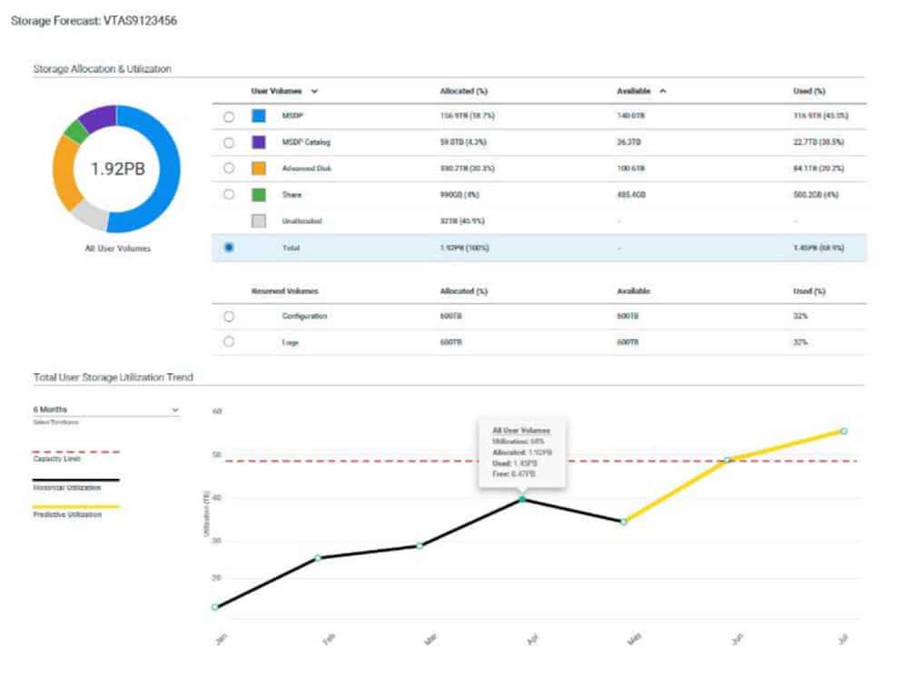
Storage forecasting

Here is a use case example of storage forecasting (at Veritas Technologies), from which the below screenshot is taken:

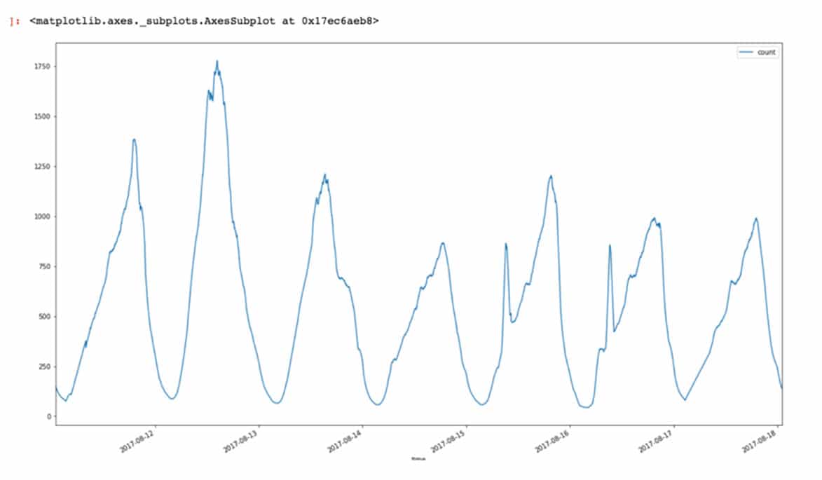
Machine learning

Here is a use case example of machine learning (at Playtech), from which the below screenshot is taken:

Overview of time series forecasting methods

Decompositional models

Time series data can exhibit a variety of patterns, so it is often helpful to split a time series into components, each representing an underlying pattern category. This is what decompositional models do.

The decomposition of time series is a statistical task that deconstructs a time series into several components, each representing one of the underlying categories of patterns. When we decompose a time series into components, we think of a time series as comprising three components: a trend component, a seasonal component, and residuals or ”noise” (containing anything else in the time series).

There are two main types of decomposition: decomposition based on rates of change and decomposition based on predictability.

Decomposition based on rates of change

This is an important time series analysis technique, especially for seasonal adjustment. It seeks to construct, from an observed time series, a number of component series (that could be used to reconstruct the original by additions or multiplications) where each of these has a certain characteristic or type of behavior.

If data shows some seasonality (e.g. daily, weekly, quarterly, yearly) it may be useful to decompose the original time series into the sum of three components:

Y(t) = S(t) + T(t) + R(t)

where S(t) is the seasonal component, T(t) is the trend-cycle component, and R(t) is the remainder component.

There are several techniques to estimate such a decomposition. The most basic one is called classical decomposition and consists in:

1. Estimating trend T(t) through a rolling mean
2. Computing S(t) as the average detrended series Y(t)-T(t) for each season (e.g. for each month)
3. Computing the remainder series as R(t)=Y(t)-T(t)-S(t)

Time series can also be decomposed into:

• T_t, the trend component at time t, which reflects the long-term progression of the series. A trend exists when there is a persistent increasing or decreasing direction in the data.</span>
• C_t, the cyclical component at time t, which reflects repeated but non-periodic fluctuations. The duration of these fluctuations is usually of at least two years.
• S_t, the seasonal component at time t, reflecting seasonality (seasonal variation). Seasonality occurs over a fixed and known time period (e.g., the quarter of the year, the month, or day of the week).
• I_t, the irregular component (“residuals” or "noise") at time t, which describes random, irregular influences.

Additive vs. multiplicative decomposition

In an additive time series, the components add together to make the time series. In a multiplicative time series, the components multiply together to make the time series.

Here is an example of a time series using an additive model:

An additive model is used when the variations around the trend do not vary with the level of the time series. To learn more about forecasting time series data based on an additive model where non-linear trends are fit with yearly, weekly, and daily seasonality, plus holiday effects, see the “Forecasting with FB Prophet and InfluxDB” tutorial which shows how to make a univariate time series prediction (Facebook Prophet is an open source library published by Facebook that is based on decomposable — trend+seasonality+holidays — models).

Here is an example of a time series using a multiplicative model:

A multiplicative model is appropriate if the trend is proportional to the level of the time series.

Decomposition based on predictability

The theory of time series analysis makes use of the idea of decomposing a time series into deterministic and non-deterministic components (or predictable and unpredictable components).

In statistics, Wold’s decomposition or the Wold representation theorem, named after Herman Wold, says that every covariance-stationary time series can be written as the sum of two time series, one deterministic and one stochastic. Formally:

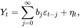
Where:

• Y_t is the time series being considered,
• E_t is an uncorrelated sequence which is the innovation process to the process — that is, a white noise process that is input to the linear filter {b_j}
• b is the possibly infinite vector of moving average weights (coefficients or parameters)
• n_t is a deterministic time series, such as one represented by a sine wave.

Types of time series methods used for forecasting

Times series methods refer to different ways to measure timed data. Common types include: - Autoregression (AR) - Moving Average (MA) - Autoregressive Moving Average (ARMA) - Autoregressive Integrated Moving Average (ARIMA) - Seasonal Autoregressive Integrated Moving-Average (SARIMA)

The important thing is to select the appropriate forecasting method based on the characteristics of the time series data.

Smoothing-based models

In time series forecasting, data smoothing is a statistical technique that involves removing outliers from a time series data set to make a pattern more visible. Inherent in the collection of data taken over time is some form of random variation. Smoothing data removes or reduces random variation and shows underlying trends and cyclic components.

Moving-average model

In time series analysis, the moving-average model (MA model), also known as moving-average process, is a common approach for modeling univariate time series. The moving-average model specifies that the output variable depends linearly on the current and various past values of a stochastic (imperfectly predictable) term.

Together with the autoregressive (AR) model (covered below), the moving-average model is a special case and key component of the more general ARMA and ARIMA models of time series, which have a more complicated stochastic structure.

Contrary to the AR model, the finite MA model is always stationary.

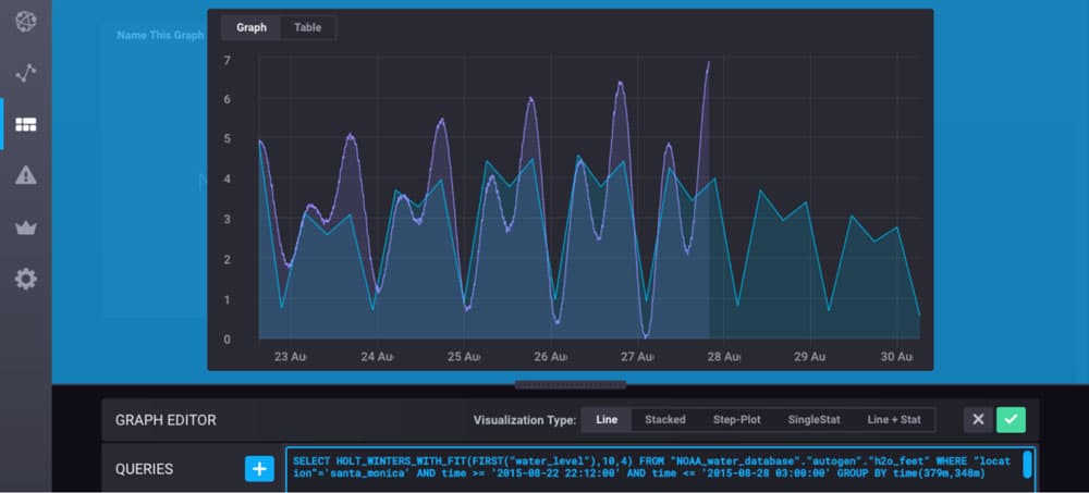
Exponential smoothing model

Exponential smoothing is a rule of thumb technique for smoothing time series data using the exponential window function. Exponential smoothing is an easily learned and easily applied procedure for making some determination based on prior assumptions by the user, such as seasonality. Different types of exponential smoothing include single exponential smoothing, double exponential smoothing, and triple exponential smoothing (also known as the Holt-Winters method). For tutorials on how to use Holt-Winters out of the box with InfluxDB, see “When You Want Holt-Winters Instead of Machine Learning” and “Using InfluxDB to Predict The Next Extinction Event”).

In single exponential smoothing, forecasts are given by:

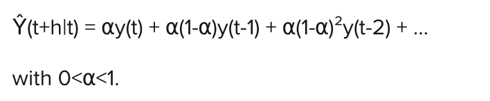
Triple Exponential Smoothing or Holt Winters is mathematically similar to Single Exponential Smoothing except that the seasonality and trend are included in the forecast.

Moving-average model vs. exponential smoothing model

• Whereas in the simple moving average the past observations are weighted equally, exponential functions are used to assign exponentially decreasing weights over time (recent observations are given relatively more weight in forecasting than the older observations).
• In the case of moving averages, the weights assigned to the observations are the same and are equal to 1/N. In exponential smoothing, however, there are one or more smoothing parameters to be determined (or estimated) and these choices determine the weights assigned to the observations.

Forecasting models including seasonality

ARIMA and SARIMA

To define ARIMA and SARIMA, it’s helpful to first define autoregression. Autoregression is a time series model that uses observations from previous time steps as input to a regression equation to predict the value at the next time step.

AutoRegressive Integrated Moving Average (ARIMA) models are among the most widely used time series forecasting techniques:

• In an Autoregressive model, the forecasts correspond to a linear combination of past values of the variable.
• In a Moving Average model the forecasts correspond to a linear combination of past forecast errors.

The ARIMA models combine the above two approaches. Since they require the time series to be stationary, differencing (Integrating) the time series may be a necessary step, i.e. considering the time series of the differences instead of the original one.

The SARIMA model (Seasonal ARIMA) extends the ARIMA by adding a linear combination of seasonal past values and/or forecast errors.

TBATS

The TBATS model is a forecasting model based on exponential smoothing. The name is an acronym for Trigonometric, Box-Cox transform, ARMA errors, Trend, and Seasonal components.

The TBATS model’s main feature is its capability to deal with multiple seasonalities by modelling each seasonality with a trigonometric representation based on Fourier series. A classic example of complex seasonality is given by daily observations of sales volumes which often have both weekly and yearly seasonality.