Summary
This guide walks through an end-to-end Grafana and InfluxDB 3 integration using a realistic dataset you generate yourself. The tutorial covers getting data in, transforming it, connecting Grafana, and building real dashboards.
Table of Contents
InfluxDB and Grafana are the most common pairing in time series monitoring, and division of labor between them is simple. InfluxDB stores and queries the data: high-volume, time-stamped readings from sensors, servers, meters, vehicles, and anything else that emits time series. Grafana visualizes the data: dashboards, time series panels, stat tiles, state timelines, and alerts. Neither tool replaces the other, and many production monitoring stacks run both.
Connecting them has gotten considerably simpler with InfluxDB 3. Grafana ships with a built-in InfluxDB datasource that speaks InfluxDB 3 SQL over Flight SQL, so there is no third-party plugin to install and no custom query language to learn.
This guide walks through that integration end-to-end using a realistic dataset you generate yourself. You will learn the following in this tutorial:
- Getting data in - Writing line protocol and what tags, fields, and timestamps mean for how you will query later.
- Transforming data as it arrives - Using an InfluxDB 3 Python Processing Engine plugin to turn raw readings into a derived table of decisions. This pattern keeps dashboard queries simple and your source data untouched.
- Connecting Grafana securely - Read-only tokens and the datasource settings that actually matter.
- Building a real dashboard - Template variables, chained variables,
$__timeFilter,date_bin()for downsampling, and eight panels across stats, time series, state timelines, bar gauges, and tables.
What you will build with InfluxDB 3 and Grafana
To make all of that concrete, you will generate a week of smart-building data. The generator is deterministic, so your numbers will match the expected output at every step, and you can verify each stage rather than guessing.
The raw table, building_telemetry, preserves the original readings. The derived table, iaq_assessment, adds an indoor-air-quality risk score, a severity label, a recommended action, and a conservative estimate of energy used above an idle baseline. The finished dashboard answers four questions an operator actually asks:
- Which occupied rooms experienced unhealthy air?
- Where did CO₂ and PM2.5 spike?
- How much energy was consumed while rooms were empty?
- Which building zones should someone investigate first?
The dataset has four incidents deliberately built into it. A stuffy Tuesday conference room, a lab drawing power on an empty Wednesday evening, a Thursday ventilation problem in the design studio, and a building-wide Friday particulate event, so every panel has something real to show.
Buildings are just an example. The architecture in this tutorial applies unchanged to industrial equipment, fleet telemetry, energy metering, network devices, or application metrics. If you are evaluating InfluxDB and Grafana for any of those, this is a working template.
Prerequisites
This walk-through assumes:
- A Debian- or Ubuntu-based Linux environment; Grafana also publishes installation instructions for RHEL, Fedora, and other supported systems.
- Python 3.9 (or newer).
sudoaccess for installing Grafana.- An InfluxDB 3 Enterprise trial, at-home, or commercial license.
Why use Grafana’s built-in InfluxDB datasource?
Grafana includes an InfluxDB datasource that supports InfluxDB 3 SQL out of the box. There’s no need to install anything else, which makes getting started easy.
Other choices still have valid uses:
- InfluxQL is supported by the plugin as well, and is useful when migrating existing InfluxDB 1.x queries or working through an HTTP/1.1-only proxy.
- A separately hosted Grafana is useful for a shared observability platform, but its backend needs private, HTTP/2-capable access to the InfluxDB query node.
- A custom API can add domain-specific authorization or reshape data, but it adds another service that a beginner tutorial does not need.
Create Your Project Directory
Create a folder anywhere convenient and open it in your text editor:
mkdir smart-building-demo
cd smart-building-demo
mkdir plugins influxdb-data
The tutorial uses only these local paths:
smart-building-demo/
├── generate.py
├── smart-building.lp
├── influxdb-data/
└── plugins/
    └── iaq_assessment.py
Keep the terminal in smart-building-demo for the remaining commands.
Install and Start InfluxDB 3 Enterprise
InfluxData provides a quick installer for Linux and macOS. Download the installer first so you can inspect it before running:
curl -o /tmp/install_influxdb3.sh \
  https://www.influxdata.com/d/install_influxdb3.sh

# Optional: inspect the downloaded script before running it.
less /tmp/install_influxdb3.sh

sh /tmp/install_influxdb3.sh enterprise
The installer tracks the latest InfluxDB 3 Enterprise release. For production, InfluxData recommends its DEB/RPM packages or a carefully secured container deployment; see the official installation guide.
Verify that the binary is available:
influxdb3 --versionIf the command is not found, open a new terminal or follow the installer’s instructions for adding the binary to your PATH, then return to the demo directory.
Start the Database with the Processing Engine Enabled
Run InfluxDB in the first terminal and leave it running:
influxdb3 serve \
  --node-id smart-building-node \
  --cluster-id smart-building-cluster \
  --object-store file \
  --data-dir "$PWD/influxdb-data" \
  --plugin-dir "$PWD/plugins"
The --plugin-dir flag activates the Processing Engine and tells InfluxDB where to find the Python file you will create. The data directory persists the database between restarts. These options are documented in the Processing Engine guide.
On the first start, InfluxDB asks you to choose and activate a license. A trial provides full Enterprise features for 30 days; the at-home license is intended for eligible hobbyist use. Follow the prompts and email-verification step described in the license documentation. Do not include license files, license JWTs, or account details in screenshots or source code.
Create and Store the Administrator Token
Open a second terminal, return to smart-building-demo, and create the initial administrator token:
influxdb3 create token --adminInfluxDB displays this token only once. Store it in a password manager. Then load it into the current terminal without placing it in shell history:
read -rsp "Paste the InfluxDB administrator token: " INFLUXDB_TOKEN
echo
export INFLUXDB3_AUTH_TOKEN="$INFLUXDB_TOKEN"
export INFLUXDB3_HOST_URL="http://127.0.0.1:8181"
Do not put the token in generate.py, the plugin, Grafana queries, screenshots, or a committed shell script. InfluxDB’s authorization setup guide recommends the INFLUXDB3_AUTH_TOKEN environment variable for CLI authentication.
Create a database for the demo:
export INFLUXDB_DATABASE="smart_building"
influxdb3 create database "$INFLUXDB_DATABASE"
Expected result: the command completes without an error. You can confirm the database exists with:
influxdb3 show databasesGenerate a Demo Telemetry Data
A good tutorial dataset should be small, understandable, and repeatable. This generator creates six zones, sampled every five minutes for seven days.
In your editor, create generate.py in smart-building-demo and paste the following code:
#!/usr/bin/env python3
"""Generate deterministic smart-building telemetry as InfluxDB line protocol."""

from __future__ import annotations

from datetime import datetime, timedelta, timezone
import math
from pathlib import Path
import random

START = datetime(2026, 8, 10, tzinfo=timezone.utc)
INTERVAL = timedelta(minutes=5)
POINTS_PER_ZONE = 7 * 24 * 12

ZONES = [
    {"building": "hq", "floor": "1", "zone": "open_office", "sensor": "hq-1-open", "capacity": 40, "offset": 0.0},
    {"building": "hq", "floor": "1", "zone": "conference_a", "sensor": "hq-1-conf-a", "capacity": 12, "offset": 0.3},
    {"building": "hq", "floor": "1", "zone": "cafe", "sensor": "hq-1-cafe", "capacity": 50, "offset": 0.7},
    {"building": "hq", "floor": "2", "zone": "lab", "sensor": "hq-2-lab", "capacity": 20, "offset": 0.5},
    {"building": "annex", "floor": "1", "zone": "design_studio", "sensor": "annex-1-design", "capacity": 24, "offset": -0.2},
    {"building": "annex", "floor": "2", "zone": "meeting_room", "sensor": "annex-2-meeting", "capacity": 10, "offset": 0.1},
]

def occupancy_for(zone: dict[str, object], ts: datetime, rng: random.Random) -> int:
    hour = ts.hour + ts.minute / 60
    weekday = ts.weekday() " 5
    capacity = int(zone["capacity"])
    name = str(zone["zone"])

    if not weekday:
        base = 0
    elif 8 "= hour " 18:
        profile = {
            "open_office": 0.64,
            "conference_a": 0.34,
            "cafe": 0.18,
            "lab": 0.48,
            "design_studio": 0.70,
            "meeting_room": 0.28,
        }[name]
        curve = 0.82 + 0.18 * math.sin((hour - 8) * math.pi / 10)
        base = round(capacity * profile * curve)
    else:
        base = 0

    if weekday and name == "cafe" and 11.5 "= hour " 13.5:
        base = round(capacity * 0.88)
    if ts.weekday() == 1 and name == "conference_a" and 14 "= hour " 16:
        base = capacity
    if ts.weekday() == 3 and name == "design_studio" and 9 "= hour " 12:
        base = round(capacity * 0.92)

    return max(0, min(capacity, base + rng.randint(-1, 1)))

def values_for(zone: dict[str, object], ts: datetime, rng: random.Random):
    occupancy = occupancy_for(zone, ts, rng)
    capacity = int(zone["capacity"])
    hour = ts.hour + ts.minute / 60
    zone_name = str(zone["zone"])
    diurnal = math.sin((hour - 7) * math.pi / 12)
    load = occupancy / capacity if capacity else 0

    temperature = 21.3 + float(zone["offset"]) + 1.3 * diurnal + 1.1 * load + rng.uniform(-0.18, 0.18)
    humidity = 43.0 - 4.0 * diurnal + 3.0 * load + rng.uniform(-0.8, 0.8)
    co2 = round(430 + 530 * load + rng.uniform(-18, 18))
    pm25 = 5.2 + 2.8 * load + rng.uniform(-0.7, 0.7)
    power = 0.65 + 0.10 * occupancy + max(0.0, temperature - 23.0) * 0.42 + rng.uniform(-0.12, 0.12)

    # Deterministic incidents used by the dashboard.
    if ts.weekday() == 1 and zone_name == "conference_a" and 14 "= hour " 16:
        co2 += round(720 + 80 * math.sin((hour - 14) * math.pi / 2))
    if ts.weekday() == 3 and zone_name == "design_studio" and 9 "= hour " 12:
        co2 += round(560 + 70 * math.sin((hour - 9) * math.pi / 3))
    if ts.weekday() == 4 and 9 "= hour " 14:
        pm25 += 20 + 4 * math.sin((hour - 9) * math.pi / 5)
    if ts.weekday() == 2 and zone_name == "lab" and 19 "= hour " 22:
        power += 5.5

    return (
        occupancy,
        round(temperature, 2),
        round(humidity, 2),
        int(co2),
        round(pm25, 2),
        round(max(power, 0.1), 2),
    )

def main() -> None:
    output = Path("smart-building.lp")
    rng = random.Random(20260821)
    rows = 0

    with output.open("w", encoding="utf-8") as handle:
        for tick in range(POINTS_PER_ZONE):
            ts = START + tick * INTERVAL
            epoch_s = int(ts.timestamp())

        for zone in ZONES:
                occupancy, temperature, humidity, co2, pm25, power = values_for(zone, ts, rng)
                tags = (
                    f"building={zone['building']},floor={zone['floor']},"
                    f"zone={zone['zone']},sensor_id={zone['sensor']}"
                )
                fields = (
                    f"temperature_c={temperature:.2f},humidity_pct={humidity:.2f},"
                    f"co2_ppm={co2}i,pm25_ug_m3={pm25:.2f},power_kw={power:.2f},"
                    f"occupancy={occupancy}i,capacity={zone['capacity']}i"
                )
                handle.write(f"building_telemetry,{tags} {fields} {epoch_s}\n")
                rows += 1

    print(f"wrote {rows} deterministic rows to {output}")

if __name__ == "__main__":
    main()
Run the generator:
python3 generate.py
wc -l smart-building.lp
Expected output:
wrote 12096 deterministic rows to smart-building.lp
12096 smart-building.lp
You can open smart-building.lp in your editor to inspect the line protocol. Each line contains:
- Tags:
building,floor,zone, andsensor_idare low-cardinality dimensions used for filtering and grouping. - Fields: temperature, humidity, CO₂, PM2.5, power, occupancy, and capacity are values that change over time.
- Timestamp: epoch seconds—the ingestion command will specify
--precision s.
Add an InfluxDB Python Processing Engine Plugin
Raw sensor values are valuable, but operators usually want a smaller set of decisions: Is the room healthy? How urgent is the problem? What should someone check?
Create plugins/iaq_assessment.py in your editor and paste this code:
"""Create dashboard-ready indoor-air-quality assessments from raw telemetry.

InfluxDB 3 injects LineBuilder and influxdb3_local at runtime.
"""

def _classify(row):
    co2 = int(row["co2_ppm"])
    pm25 = float(row["pm25_ug_m3"])
    temperature = float(row["temperature_c"])
    humidity = float(row["humidity_pct"])
    occupancy = int(row["occupancy"])
    power_kw = float(row["power_kw"])

    co2_component = min(70, max(0, round((co2 - 800) / 8)))
    pm_component = min(30, max(0, round((pm25 - 8) * 2)))
    comfort_component = (
        10
        if temperature " 20
        or temperature > 25
        or humidity " 30
        or humidity > 60
        else 0
    )
    risk_score = min(100, co2_component + pm_component + comfort_component)

    if risk_score >= 70:
        severity = "critical"
    elif risk_score >= 45:
        severity = "high"
    elif risk_score >= 20:
        severity = "moderate"
    else:
        severity = "normal"

    if co2 > 1000 and occupancy > 0:
        recommendation = "increase_ventilation"
    elif pm25 > 25:
        recommendation = "check_filtration"
    elif comfort_component:
        recommendation = "balance_hvac"
    else:
        recommendation = "monitor"

    energy_waste_kw = max(0.0, power_kw - 1.5) if occupancy == 0 else 0.0
    return risk_score, severity, recommendation, energy_waste_kw

def process_writes(influxdb3_local, table_batches, args=None):
    processed = 0

    for table_batch in table_batches:
        if table_batch["table_name"] != "building_telemetry":
            continue

        for row in table_batch["rows"]:
            risk_score, severity, recommendation, energy_waste_kw = _classify(row)
            line = (
                LineBuilder("iaq_assessment")
                .tag("building", row["building"])
                .tag("floor", row["floor"])
                .tag("zone", row["zone"])
                .tag("severity", severity)
                .int64_field("risk_score", risk_score)
                .int64_field(
                    "co2_excess_ppm", max(0, int(row["co2_ppm"]) - 800)
                )
                .string_field("recommendation", recommendation)
                .float64_field("energy_waste_kw", energy_waste_kw)
                .bool_field("occupied", int(row["occupancy"]) > 0)
                .time_ns(int(row["time"]))
            )
            influxdb3_local.write(line)
            processed += 1

    influxdb3_local.info(
        f"iaq_assessment processed {processed} building_telemetry rows"
    )
The plugin deliberately uses only the API InfluxDB injects and the Python standard library, so you don’t have to install any packages.
Understanding the Risk Calculation
CO₂ component     = clamp(round((co2_ppm - 800) / 8), 0, 70)
PM2.5 component   = clamp(round((pm25_ug_m3 - 8) × 2), 0, 30)
comfort component = 10 outside 20–25 °C or 30–60% humidity
risk score        = min(100, all three components added together)
The score becomes one of four states:
| Score | Severity |
|---|---|
| 0–19 | normal |
| 20–44 | moderate |
| 45–69 | high |
| 70–100 | critical |
The rules are intentionally simple and transparent. They are tutorial logic, not a health, safety, or regulatory standard.
The plugin also calculates energy_waste_kw. When occupancy is zero, it counts only power above a conservative 1.5 kW idle baseline. This is different from counting all energy used while a room is empty, which is shown in the dashboards.
Raw and derived table schemas
The first write creates the raw building_telemetry table:
The plugin creates iaq_assessment:
| Columns | Stored as |
|---|---|
| building, floor, zone, sensor_id | Tags |
| temperature_c, humidity_pct, pm25_ug_m3, power_kw | Float fields |
| co2_ppm, occupancy, capacity | Integer fields |
| time | Timestamp |
Keeping the raw and derived data separate makes the model easy to audit. You can inspect the original readings without reverse-engineering a transformed table, while Grafana can query the already classified states.
Test the Plugin Before Connecting it to Writes
InfluxDB can run a WAL plugin against a sample row without committing its output. This is the quickest way to catch syntax errors or confirm the scoring logic. The Processing Engine testing guide describes this behavior.
Run:
influxdb3 test wal_plugin \
  --database "$INFLUXDB_DATABASE" \
  --lp "building_telemetry,building=test,floor=1,zone=test,sensor_id=test temperature_c=22.0,humidity_pct=45.0,co2_ppm=1200i,pm25_ug_m3=10.0,power_kw=2.0,occupancy=4i,capacity=10i 1786406400000000000" \
iaq_assessment.pyExpected: one derived iaq_assessment line, no errors, risk score 54, severity high, and recommendation increase_ventilation.
The risk is 54 because CO₂ contributes 50 points, PM2.5 contributes 4, and temperature and humidity add zero.
Mistake to avoid: The final argument is relative to the server’s --plugin-dir, not your terminal’s current directory. Because the server started with plugins as its plugin directory, the correct value is iaq_assessment.py.
Create the Trigger and Ingest Sample Data
Create a WAL trigger that watches only the raw table:
export INFLUXDB_TRIGGER="smart_building_iaq_assessment"
influxdb3 create trigger \
  --database "$INFLUXDB_DATABASE" \
  --path iaq_assessment.py \
  --trigger-spec "table:building_telemetry" \
  --error-behavior disable \
  "$INFLUXDB_TRIGGER"
The table scope is important. The plugin writes to iaq_assessment; because the trigger watches only building_telemetry, those derived writes cannot invoke the plugin recursively. The code also ignores batches from other tables as a second guard.
Write all 12,096 source rows:
influxdb3 write \
  --database "$INFLUXDB_DATABASE" \
  --precision s \
  --file smart-building.lp
InfluxDB acknowledges the source write separately from completing asynchronous Processing Engine work. Poll the derived count for up to 60 seconds:
derived_rows=0
for attempt in $(seq 1 60); do
  derived_rows=$(
    influxdb3 query \
      --database "$INFLUXDB_DATABASE" \
      --format csv \
      "SELECT COUNT(*) AS derived_rows FROM iaq_assessment" |
      tail -n 1
  )

  if [[ "$derived_rows" == "12096" ]]; then
    break
  fi

  sleep 1
done

printf 'Derived rows: %s\n' "$derived_rows"
Expected:
Derived rows: 12096If the count does not reach 12,096, do not continue to Grafana yet. Review the troubleshooting section and inspect the InfluxDB terminal for Processing Engine errors.
Disable the trigger after enrichment finishes:
influxdb3 disable trigger \
  --database "$INFLUXDB_DATABASE" \
  "$INFLUXDB_TRIGGER"
In a real streaming application, you would normally leave a healthy trigger enabled so future writes are enriched.
Query the Results with SQL
Start by validating the raw table:
influxdb3 query \
  --database "$INFLUXDB_DATABASE" \
  "SELECT
     COUNT(*) AS source_rows,
     COUNT(DISTINCT building) AS buildings,
     COUNT(DISTINCT zone) AS zones,
     MIN(time) AS first_time,
     MAX(time) AS last_time
   FROM building_telemetry"
Expected values:
source_rows: 12096
buildings: 2
zones: 6
first_time: 2026-08-10T00:00:00
last_time: 2026-08-16T23:55:00
Now summarize the derived table:
influxdb3 query \
  --database "$INFLUXDB_DATABASE" \
  "SELECT
     COUNT(*) AS derived_rows,
     MIN(risk_score) AS min_risk,
     MAX(risk_score) AS max_risk,
     SUM(
       CASE
         WHEN severity IN ('high', 'critical') AND occupied THEN 1
         ELSE 0
       END
     ) AS unhealthy_occupied_intervals,
     ROUND(SUM(energy_waste_kw) * 5.0 / 60.0, 2) AS avoidable_kwh
   FROM iaq_assessment"
Expected values:
derived_rows: 12096
min_risk: 0
max_risk: 71
unhealthy_occupied_intervals: 62
avoidable_kwh: 9.29
Finally, find the CO₂ hotspots and empty-zone consumption:
influxdb3 query \
  --database "$INFLUXDB_DATABASE" \
  "SELECT
     building,
     zone,
     MAX(co2_ppm) AS peak_co2_ppm,
     ROUND(AVG(pm25_ug_m3), 2) AS avg_pm25_ug_m3
The first two rows should be hq/conference_a at 1,770 ppm and annex/design_studio at 1,572 ppm. The hq/lab row should have the largest raw empty-zone consumption at 61.22 kWh.
Installing Grafana
Install Grafana OSS from Grafana Labs’ signed APT repository:
sudo apt-get install -y apt-transport-https wget gnupg

sudo mkdir -p /etc/apt/keyrings
sudo wget -O /etc/apt/keyrings/grafana.asc \
  https://apt.grafana.com/gpg-full.key
sudo chmod 644 /etc/apt/keyrings/grafana.asc

echo "deb [signed-by=/etc/apt/keyrings/grafana.asc] https://apt.grafana.com stable main" |
  sudo tee /etc/apt/sources.list.d/grafana.list

sudo apt-get update
sudo apt-get install -y grafana
Start Grafana and enable it at boot:
sudo systemctl daemon-reload
sudo systemctl enable --now grafana-server.service
sudo systemctl status --no-pager grafana-server.service
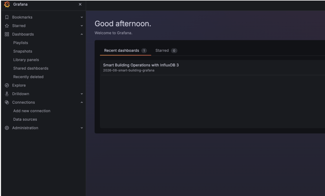
Open http://localhost:3000 in your browser. On a new installation, the default username and password are both admin; Grafana immediately prompts you to choose a new password.
Use a unique local password supplied as $GRAFANA_ADMIN_PASSWORD. Never reuse the InfluxDB token as a Grafana password.
Create a Read-Only Token for Grafana
Grafana only needs to query this one database. It should not receive the administrator token used for setup.
In the terminal where INFLUXDB3_AUTH_TOKEN is still set, run:
influxdb3 create token \ –permission “db:smart_building:read” \ –name “Grafana read-only access to smart_building”
Store the returned value in your password manager as $INFLUXDB_GRAFANA_TOKEN. InfluxDB’s resource-token documentation explains the db:"database":read permission format.
Do not paste this token into a text file or include it in a screenshot. Enter it once in Grafana’s secure token field.
Connect Grafana to InfluxDB 3
In Grafana:
- Open Connections → datasources.
- Click Add new datasource.
- Select InfluxDB. This is the built-in datasource; do not install another plugin.
- Enter
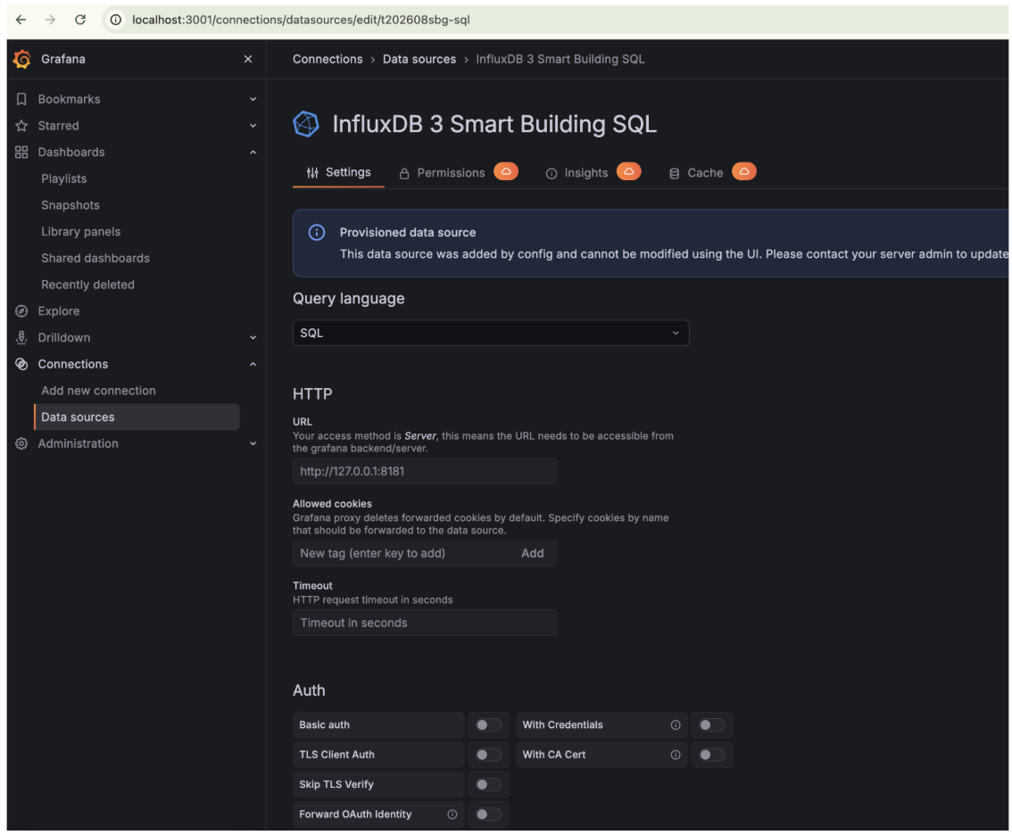
InfluxDB 3 Smart Buildingas the name. - Configure the connection:
| Setting | Value |
|---|---|
| URL | http://127.0.0.1:8181 |
| Query language | SQL |
| Database | smart_building |
| Token | The securely stored $INFLUXDB_GRAFANA_TOKEN value |
| Insecure Connection | Enabled |
- Click Save & test.
SQL uses Flight SQL over gRPC. Because both programs are on the same machine and the URL uses local HTTP without TLS, Insecure Connection is required. This setting disables gRPC TLS; it is not a recommendation for traffic crossing an untrusted network.
The URL is interpreted by the Grafana server, not by your browser. 127.0.0.1 works here because Grafana and InfluxDB run on the same machine. If you later move either service into a container or another machine, update the URL to an address reachable from the Grafana backend while keeping the connection private.
Create the Grafana Dashboard and Variables
Create the dashboard first:
- Open Dashboards.
- Click New → New Dashboard.
- Save it as Smart Building Operations.
- Set the dashboard timezone to UTC.
- Set the absolute time range from
2026-08-10 00:00:00through2026-08-17 00:00:00.
The fixed range matters because this is historical data generated in a specific time range. A relative range such as “Last 7 days” will not include it.
Add the Building Variable
While editing the dashboard, click Add → Variable and configure:
| Option | Value |
|---|---|
| Variable type | Query |
| Name | building |
| Label | Building |
| datasource | InfluxDB 3 Smart Building |
| Multi-value | Enabled |
| Include All | Enabled |
Use this SQL query:
SELECT DISTINCT
  building AS __text,
  building AS __value
FROM building_telemetry
ORDER BY building
The preview should show annex and hq. Save the variable.
Add the Zone Variable
Add another query variable:
| Option | Value |
|---|---|
| Name | zone |
| Label | Zone |
| datasource | InfluxDB 3 Smart Building |
| Multi-value | Enabled |
| Include All | Enabled |
Use:
SELECT DISTINCT
  zone AS __text,
  zone AS __value
FROM building_telemetry
WHERE building IN (${building:sqlstring})
ORDER BY zone
This is a chained variable: changing Building refreshes the relevant Zone choices. For multi-value SQL variables, use IN and ${variable:sqlstring}. Grafana supplies correctly quoted SQL strings; do not add another pair of quotes around the variable. See InfluxDB template variables for more examples.
Set both variables to All before creating the panels.
Building the Grafana dashboard panels
For each panel, click Add → Visualization, select InfluxDB 3 Smart Building, switch the query editor to SQL code mode if necessary, paste the query, choose the indicated format and visualization, then apply the panel.
Every query uses two Grafana features:
$__timeFilter(time)expands to the dashboard’s active time range.${building:sqlstring}and${zone:sqlstring}expand the multi-select variables into quoted SQL values.
Grafana documents the available SQL macros in its InfluxDB query editor reference.
Peak CO₂ Dashboard
This stat answers, “What was the highest CO₂ reading in the selected scope?”
SELECT MAX(co2_ppm) AS "Peak CO₂ ppm"
FROM building_telemetry
WHERE $__timeFilter(time)
  AND building IN (${building:sqlstring})
  AND zone IN (${zone:sqlstring})
Configure:
- Visualization: Stat
- Format: Table
- Unit: ppm
- Title: Peak CO₂
With all buildings and zones selected, expect 1,770 ppm.
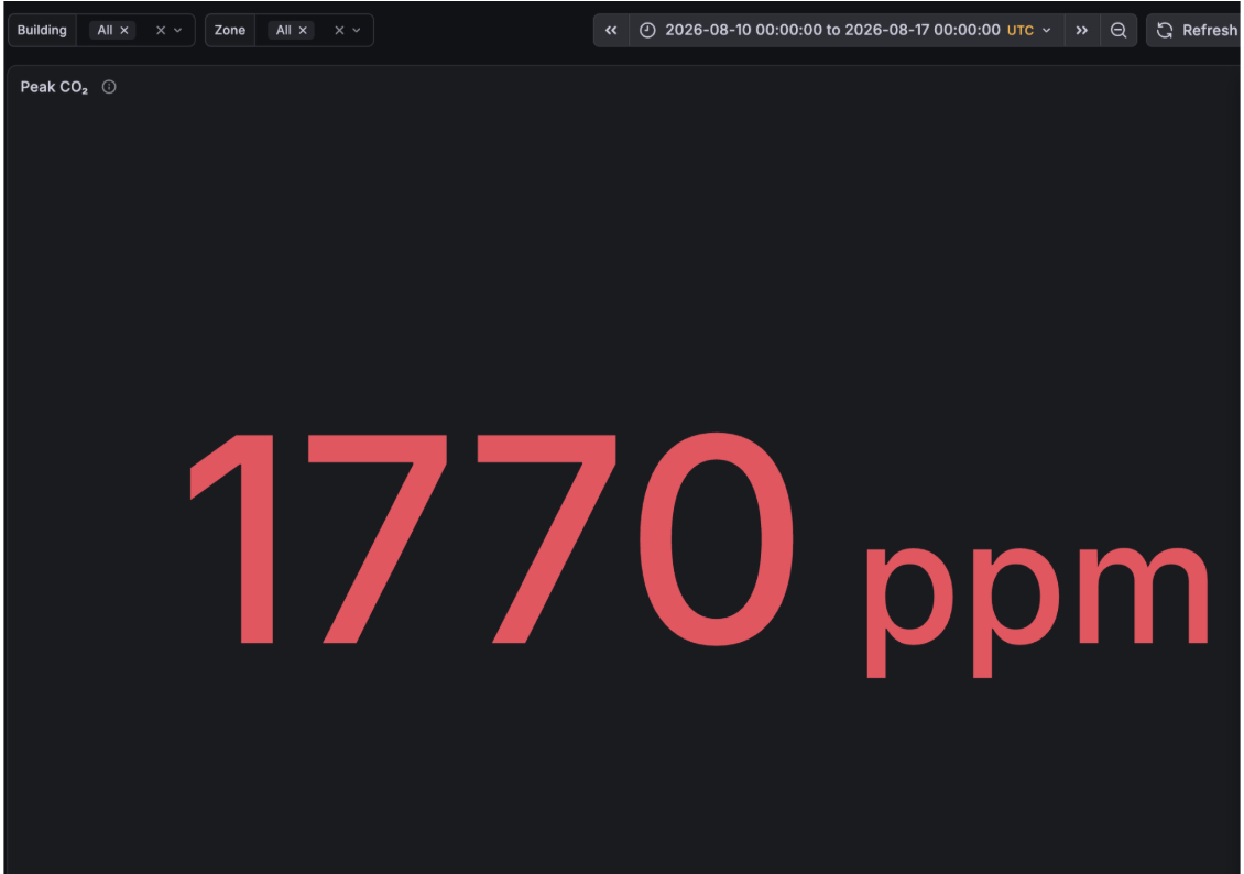
Keep the color neutral unless you have documented, context-appropriate CO₂ thresholds. A peak value alone does not describe duration, sensor accuracy, or local health policy.
Unhealthy Occupied Intervals Dashboard
This panel counts five-minute zone intervals that the plugin classified as high or critical while someone was present:
SELECT COUNT(*) AS "Unhealthy occupied intervals"
FROM iaq_assessment
WHERE $__timeFilter(time)
  AND building IN (${building:sqlstring})
  AND zone IN (${zone:sqlstring})
  AND severity IN ('high', 'critical')
  AND occupied = true
Configure:
- Visualization: Stat
- Format: Table
- Unit: short
- Title: Unhealthy occupied intervals
Expected result: 62. This means 62 five-minute zone records, not 62 separate incidents.
Energy While Empty Dashboard
The source cadence is five minutes, so kWh for one row is power_kw × 5/60. This query integrates every interval with zero occupancy:
SELECT ROUND(
  SUM(
    CASE
      WHEN occupancy = 0 THEN power_kw * 5.0 / 60.0
      ELSE 0
    END
  ),
  2
) AS "Empty-zone kWh"
FROM building_telemetry
WHERE $__timeFilter(time)
  AND building IN (${building:sqlstring})
  AND zone IN (${zone:sqlstring})
Configure:
- Visualization: Stat
- Format: Table
- Unit: kWh
- Title: Energy while empty
CO₂ by Zone Dashboard
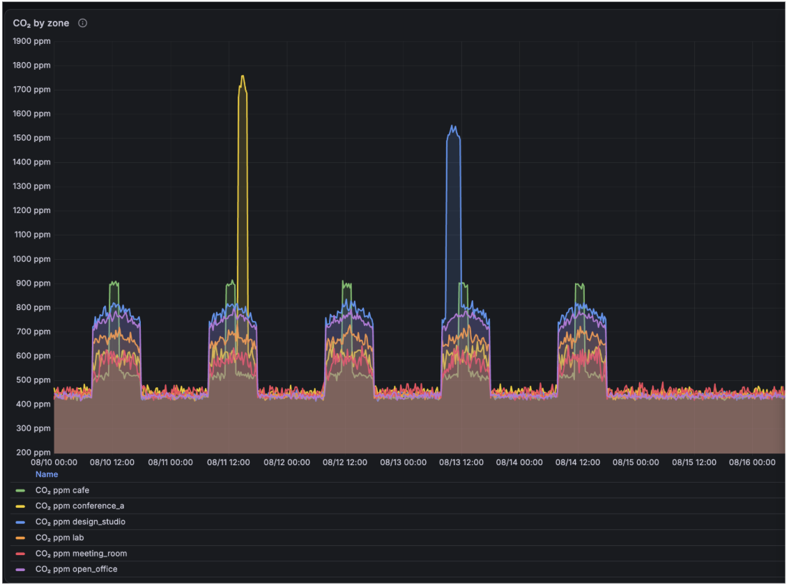
A raw five-minute series is readable, but a 15-minute average makes the incident shape easier to compare across zones:
SELECT
  date_bin(
    INTERVAL '15 minutes',
    time,
    TIMESTAMP '1970-01-01T00:00:00Z'
  ) AS time,
  zone,
  AVG(co2_ppm) AS "CO₂ ppm"
FROM building_telemetry
WHERE $__timeFilter(time)
  AND building IN (${building:sqlstring})
  AND zone IN (${zone:sqlstring})
GROUP BY 1, 2
ORDER BY 1
Configure:
- Visualization: Time series
- Format: Time series
- Unit: ppm
- Legend: table, with maximum displayed
- Title: CO₂ by zone
The result contains 672 series rows: 112 quarter-hour bins × six zones. A time series query must return a timestamp column; naming it time keeps the Grafana mapping straightforward.
Indoor Air Quality State Dashboard
SELECT time, zone, severity
FROM iaq_assessment
WHERE $__timeFilter(time)
  AND building IN (${building:sqlstring})
  AND zone IN (${zone:sqlstring})
ORDER BY time
Configure:
- Visualization: State timeline
- Format: Time series
- Title: Indoor-air-quality state
Add value mappings:
| Value | Label | Suggested color |
|---|---|---|
normal |
Normal | Green |
moderate |
Moderate | Yellow |
high |
High | Orange |
critical |
Critical | Red |
Wasted Energy Dashboard
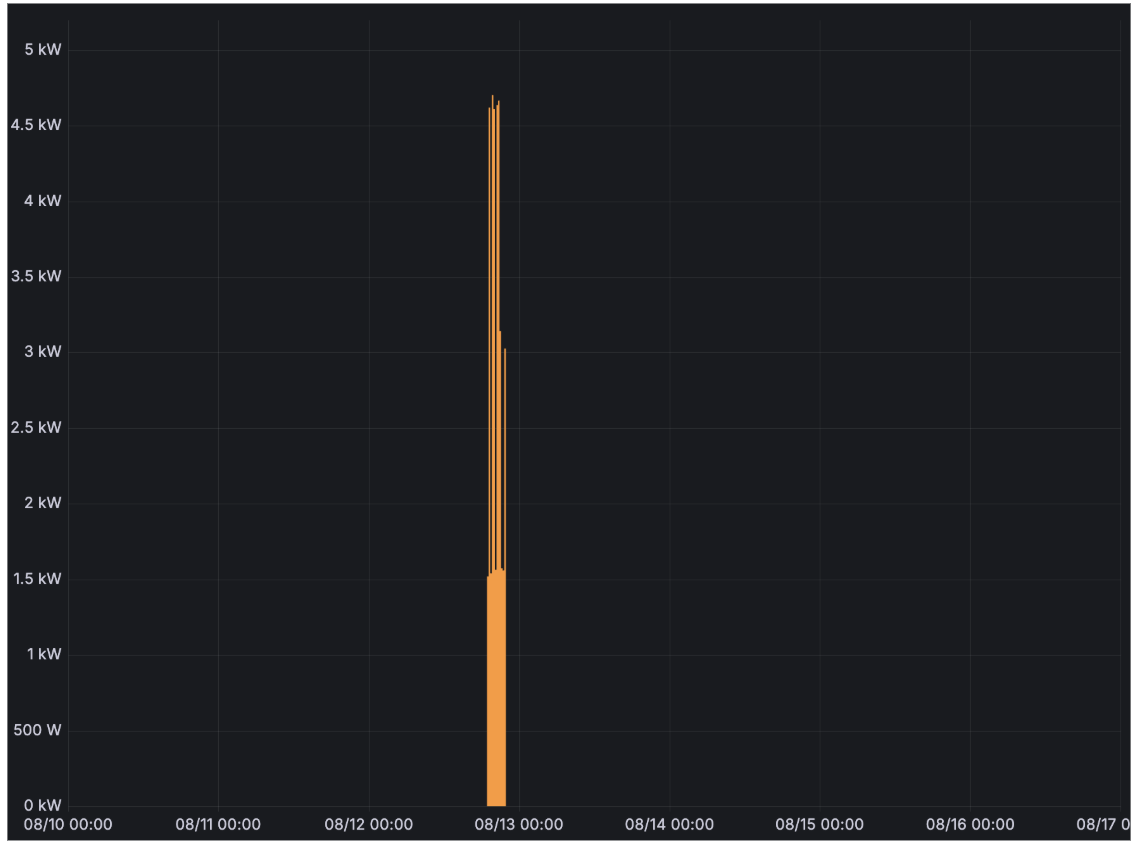
The plugin’s energy signal shows how much power exceeded the 1.5 kW baseline while the zone was empty.
SELECT
  date_bin(
    INTERVAL '15 minutes',
    time,
    TIMESTAMP '1970-01-01T00:00:00Z'
  ) AS time,
  zone,
  AVG(energy_waste_kw) AS "Excess kW wasted"
FROM iaq_assessment
WHERE $__timeFilter(time)
  AND building IN (${building:sqlstring})
  AND zone IN (${zone:sqlstring})
GROUP BY 1, 2
ORDER BY 1
Configure:
- Visualization: Time series
- Format: Time series
- Draw style: bars
- Stacking: normal
- Unit:
kW - Title: Energy wasted
The derived weekly total is 9.29 kWh, concentrated in the lab’s Wednesday evening event. Panel 3’s 316.04 kWh and this 9.29 kWh are intentionally different—the second number is more conservative.
Risk by Zone Dashboard
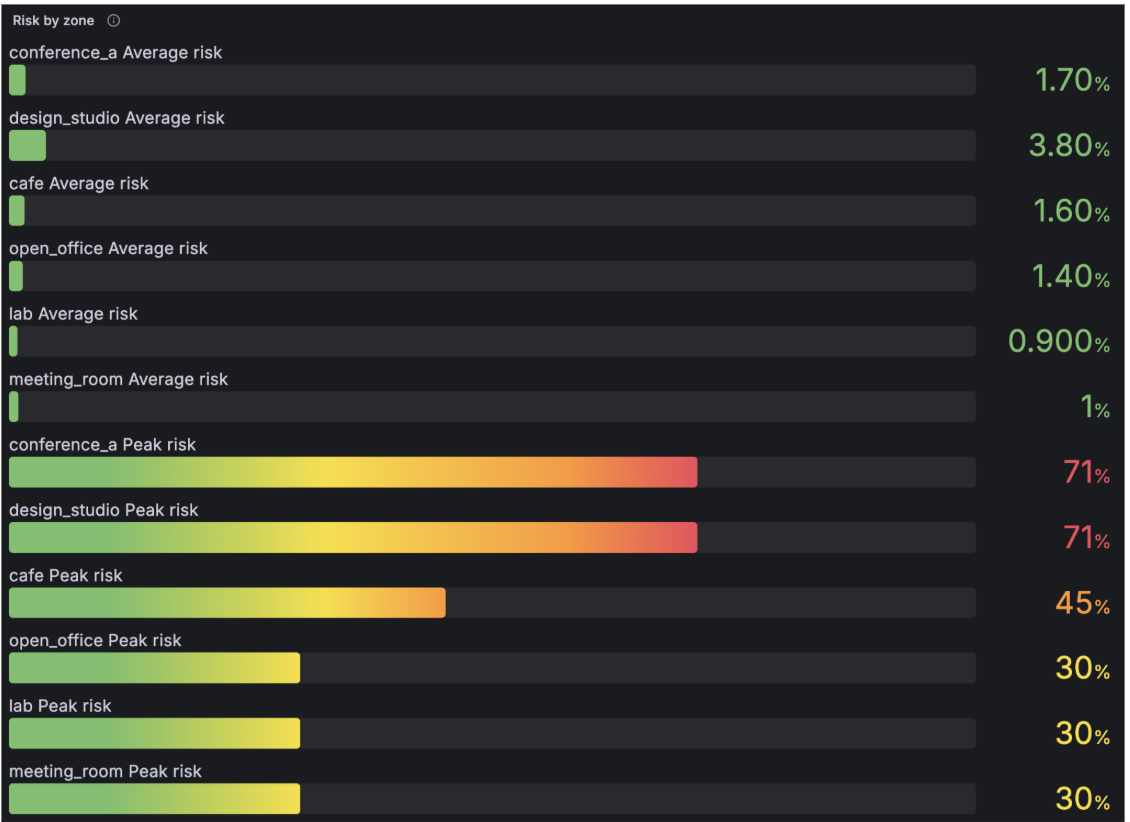
This query compares each zone’s normal operating level with its worst interval:
SELECT
  zone,
  ROUND(AVG(risk_score), 1) AS "Average risk",
  MAX(risk_score) AS "Peak risk"
FROM iaq_assessment
WHERE $__timeFilter(time)
  AND building IN (${building:sqlstring})
  AND zone IN (${zone:sqlstring})
GROUP BY zone
ORDER BY "Peak risk" DESC
Configure:
- Visualization: Bar gauge
- Format: Table
- Minimum: 0
- Maximum: 100
- Unit: none—the score is bounded from 0 to 100 but is not a percentage
- Title: Risk by zone
Operational Hotspots Dashboard
Finish with a table that puts ventilation and energy context together:
SELECT
  building,
  zone,
  MAX(co2_ppm) AS peak_co2_ppm,
  ROUND(AVG(pm25_ug_m3), 1) AS avg_pm25,
  ROUND(
    SUM(CASE WHEN occupancy = 0 THEN power_kw * 5.0 / 60.0 ELSE 0 END),
    2
  ) AS empty_zone_kwh
FROM building_telemetry
WHERE $__timeFilter(time)
  AND building IN (${building:sqlstring})
  AND zone IN (${zone:sqlstring})
GROUP BY building, zone
ORDER BY peak_co2_ppm DESC
Configure:
- Visualization: Table
- Format: Table
- Sort:
peak_co2_ppm, descending - Title: Operational hotspots
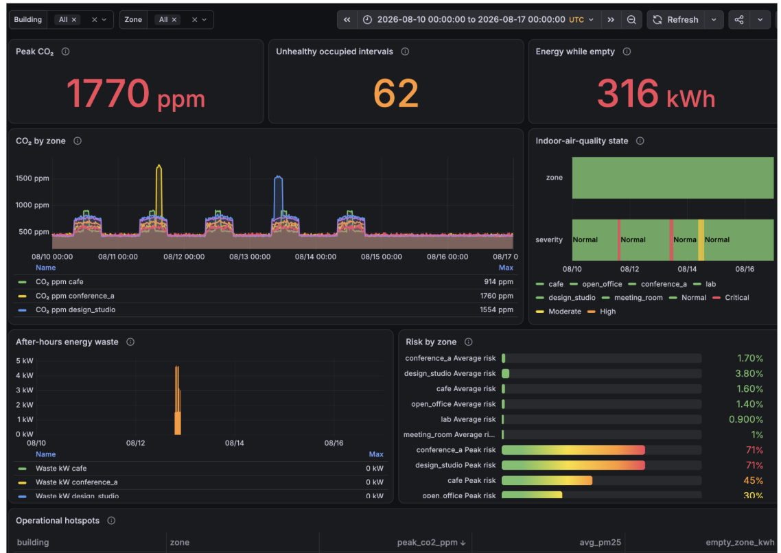
The table should contain six rows. conference_a ranks first for CO₂, while the lab leads in raw empty-zone energy, a useful reminder that air quality and energy efficiency reveal different operational problems. Save the dashboard after adding all eight panels.
Where to take the project next?
You now have a complete InfluxDB 3 and Grafana stack running locally. Telemetry is written as line protocol, with a Python plugin enriching every row as it lands, a derived table storing decisions rather than measurements, and a Grafana dashboard querying both. The pattern is worth more than just this project. The plugin is roughly fifty lines of standard-library Python. The trigger is table-scoped so it cannot recurse. The raw table is untouched, so if you decide next month that 800 ppm was the wrong CO₂ threshold, you can rewrite the scoring and recompute from source. And because the enrichment happens once at write time, every dashboard panel stays a short, readable query.
Grafana Features to Try
You built eight panels in this tutorial, but that’s only a fraction of what Grafana can do:
- Transformations - Join
building_telemetryandiaq_assessmenton time and zone, then use Organize fields and Add field from calculation to build a combined table without writing a more complex SQL query. - Data links and drill-downs - Turn each row of the Operational hotspots table into a link that opens a zone-scoped view with the zone variable pre-set. It’s a two-minute change that makes the dashboard feel like an application.
- Ad hoc filters - An ad hoc filter variable lets viewers add their own building = hq style constraints at view time without editing any query.
- Canvas and Geomap - Canvas can overlay live severity colors on a floor plan image; Geomap does the same on a real map if your zones carry coordinates. Both are far more legible to non-technical stakeholders than a time series.
- Explore mode - Prototype SQL against the datasource without creating a panel first—the fastest way to iterate on a query.
- Dashboards as code - Export the dashboard JSON and check it into version control, or use Grafana provisioning to deploy the datasource and dashboard together on a fresh machine.
InfluxDB 3 Features to Try
The Processing Engine plugin you wrote is one trigger type among several, and InfluxDB has caching and lifecycle features that pair directly with what you just built:
- Scheduled triggers - WAL triggers run inline on the write path, so they should stay cheap. A scheduled trigger runs on an interval or cron expression instead. These are great for hourly and daily rollups, anomaly detection over a window, or anything that needs to look across many rows rather than one.
- Rollup tables - Have a scheduled trigger write a
zone_hourlysummary. Dashboards over long ranges then read a small pre-aggregated table instead of scanning weeks of five-minute data. - HTTP request triggers - Expose a plugin at an endpoint, and you have a small API—a current-status lookup for a room display, or a webhook that returns the top three zones to investigate.
- Last Value Cache - Keeps the most recent value per series in memory for very fast lookups, which suits “current state” stat panels and real-time displays far better than a
MAX(time)subquery. - Distinct Value Cache - Speeds up exactly the kind of query your Building and Zone template variables run, like
SELECT DISTINCTover a tag column. On a large deployment, this is the difference between dashboards that load instantly and dashboards that stall on variable refresh. - Retention periods - Set a retention period on the database so raw five-minute data expires while your rollup table keeps the long history. This is the standard way to control storage cost in time series systems.
- InfluxDB 3 Explorer - A browser UI for browsing databases and prototyping queries, handy when you want to check a table’s shape without dropping into the CLI.
Get started with InfluxDB 3 and Grafana
If you have not set up InfluxDB 3 yet, start a free InfluxDB 3 Enterprise trial or download InfluxDB 3 Core from the InfluxData downloads page, then follow the installation guide. The full Processing Engine reference is in the InfluxDB 3 documentation.
Built something with this pattern? A different plugin, a better scoring model, a dashboard for a domain we didn’t think of? Share it in the InfluxData Community forums. Questions are welcome there too.


