Table of Contents
Time series analysis is the process of examining observations recorded over time to identify trends, seasonal patterns, relationships, and unusual changes. It accounts for the order of observations and dependencies between them. Common techniques include visualization, smoothing, decomposition, and autocorrelation analysis. These techniques help explain historical behavior, monitor systems, and prepare data for forecasting future values.
What is time series analysis?
Time series analysis studies how a measurement or event sequence changes over time. A series combines observation times with values and, where needed, an entity identifier such as a server, sensor, or location. Examples include daily sales, hourly temperature, minute-by-minute CPU usage, and timestamped application events.
The order matters: shuffling observations would remove information about trends, recurring patterns, and relationships between earlier and later values. The NIST introduction to time series analysis explains why temporal structure, including autocorrelation and seasonal variation, needs to be accounted for.
Analysis supports several distinct goals:
- Description: summarize what changed and when.
- Monitoring: recognize unusual changes against an expected baseline.
- Forecasting preparation: identify patterns and data issues before estimating future values.
- Comparison: examine relationships between measurements over aligned time periods.
A timestamp does not need to be the only field identifying a record. Multiple servers can report values at the same time, creating separate series. Measurements may be numeric, while timestamped events can also contain text, Boolean values, and other attributes.
Does time series data need regular intervals?
Time series data can be recorded at regular intervals, such as a temperature reading every minute, or irregular intervals, such as a log entry when an event occurs. Regular sampling is an assumption of many common forecasting methods, rather than a requirement for all time series data.

Irregular events can still be analyzed and modeled. One approach is to count events within fixed windows, such as errors per minute. Forecasting those counts requires a method suited to the data, especially when many windows contain zero events. See forecasting time series of counts and intermittent demand.
How does time series data differ from cross-sectional and panel data?
The distinction depends on which entities are observed and whether observations repeat over time.
| Data structure | Entities and observation times | Example |
|---|---|---|
| Time series | Observations of one entity or a defined aggregate over multiple times. | Hourly temperature at one weather station. |
| Cross-sectional | Observations of multiple entities at one time or reference period. | Temperature at several weather stations at noon. |
| Panel (longitudinal) | Repeated observations of the same multiple entities over time. | Hourly temperature at the same weather stations for a month. |
A collection of timestamped server measurements may contain many individual time series and also be organized as a panel. Entity identifiers help separate those series; their presence does not make temporal analysis irrelevant.
What patterns should you look for in time series data?
Look for changes in level, repeating patterns, relationships across lags, and observations that depart from expected behavior. The following concepts help distinguish those features.
| Concept | Meaning | Example |
|---|---|---|
| Trend | A sustained change in the level of a series. | Average server traffic grows over several months. |
| Seasonality | A pattern that repeats at a known, fixed period. | Traffic peaks during business hours each day. |
| Cycle | A rise and fall whose duration is not necessarily fixed. | Demand changes during an economic expansion and contraction. |
| Autocorrelation | The relationship between a series and its values at earlier lags. | CPU usage in one minute is related to usage in the previous minute. |
| Residuals | What remains after fitting a model or removing estimated components. | A traffic spike remains after accounting for the usual daily pattern. |
In time series decomposition, an observed series is often represented using trend-cycle, seasonal, and remainder components. The remainder is not necessarily random noise: a remaining pattern can indicate an incomplete model or a useful signal.
Seasonality can be daily, weekly, annual, or another fixed period relevant to the process. For example, a daily traffic pattern differs from an economic cycle with an uncertain duration.
What is stationarity, and why does it matter?
Stationarity means that a series’ statistical properties do not depend on when it is observed. For weak stationarity, the mean and variance are constant, and covariance depends on the lag between observations rather than their absolute times.
A trend, seasonal pattern, or changing variance can violate stationarity. Some models need a stationary series or stationary transformed series; other models explicitly represent changing level, trend, and seasonality.
Differencing compares consecutive observations and can help remove a changing level. Seasonal differencing compares observations one seasonal period apart. Transformations may help stabilize variance. Apply these only when appropriate for the method and data: unnecessary differencing can introduce false dynamics. See stationarity and differencing.
How do you analyze time series data?
A useful analysis starts with a clear question and a reproducible sequence of data checks, exploration, and validation.
- Define the objective: Decide whether you are explaining a historical change, detecting anomalies, or forecasting a specific horizon. Identify the measurement, entities, units, and decision the analysis will support.
- Check timestamps and data quality: Sort each series by time. Confirm time zones, sampling frequency, duplicate handling, missing values, and late-arriving observations. Distinguish an actual zero from a missing measurement.
- Choose an appropriate interval: Decide whether to keep raw observations or aggregate them. Use a sum for quantities such as sales totals, and an appropriate average or percentile for measurements such as utilization or latency. Aggregation can hide short spikes.
- Plot the series: Display time on the horizontal axis and the measurement on the vertical axis. Inspect shifts, gaps, outliers, trends, and repeating patterns. Compare entities separately before combining them.
- Investigate temporal structure: Examine seasonality, autocorrelation, and stationarity as relevant to the selected method. Compare similar hours or weekdays when a repeating pattern affects the baseline.
- Select and apply a method: Start with an understandable baseline, then add complexity when it improves the result. Document preprocessing and model assumptions.
- Validate and monitor: Check residuals and investigate flagged anomalies. For forecasting, test on later observations that were unavailable during training, compare with a simple baseline, and monitor performance as new data arrives.
Time series cross-validation uses training observations that precede each test observation. A rolling forecasting origin repeats this evaluation at later points in time. Match the test horizon to the real forecasting task.
Which time series analysis methods should you use?
Choose a method according to the question and the series’ structure. Describing a trend, detecting an unusual observation, and predicting tomorrow’s value require different outputs.
| Method | Purpose and useful situation | Main limitation |
|---|---|---|
| Smoothing | A moving average or exponential smoothing reduces short-term variation to reveal the underlying level or trend. | Can hide spikes and lag sudden changes; a smoother alone is not a complete forecasting model. |
| Decomposition | Separates trend-cycle, seasonal, and remainder components to explain recurring behavior. | The period and decomposition method must suit the data; changing patterns can complicate interpretation. |
| Autocorrelation analysis | Compares a series with its past values to investigate persistence and recurring lags. | A strong correlation does not establish causation; trends can distort interpretation. |
| Anomaly detection | Flags observations that differ from an expected baseline, such as unusual latency or event counts. | Results depend on the baseline and threshold; unusual observations are not automatically errors. |
| ETS models | Exponential smoothing models describe error, trend, and seasonal components for forecasting. | The chosen model must match the series; sudden structural changes can make past patterns unreliable. |
| ARIMA and seasonal ARIMA | Model dependence on past values and forecast errors, with differencing when appropriate. | Require suitable model assumptions and diagnostics; differencing too much can introduce misleading dynamics. |
The forecasting references for ETS and ARIMA explain their different approaches. Holt-Winters is a seasonal exponential smoothing method, while ETS means error, trend, and seasonal, rather than “Error, Trend, Seasonality Forecast.”
For signals such as vibration or electrical activity, spectral analysis can reveal dominant frequencies. Time-domain methods examine behavior over time and across lags. These are complementary ways of studying a signal, rather than a ranking of methods.
How does time series analysis differ from forecasting?
Time series analysis describes and investigates observed behavior. Forecasting estimates values beyond the observed period. Analysis can support forecasting, but monitoring a system or explaining a historical change does not always require a forecast.
A forecast should state its horizon, assumptions, and uncertainty. Compare a model with a simple baseline, such as the most recent observation or the value from the same period in the previous seasonal cycle. Evaluate performance on unseen later data using a suitable measure such as mean absolute error (MAE) or root mean squared error (RMSE).
Historical patterns do not guarantee future outcomes. A product launch, outage, policy change, or other structural break can change the process generating the data. Reassess models when those conditions change. Explore additional time series forecasting methods.
What are practical examples of time series analysis?
Time series analysis connects a measurement’s behavior with a specific operational question. These examples show how the same principles apply across domains.
Weather - how does temperature change during the day?
Hourly temperature measurements reveal daily variation and differences between measured and “feels like” temperature. Longer histories support comparisons across seasons. A short observation period alone does not establish a reliable weather forecast.

Infrastructure - is server activity following its usual pattern?
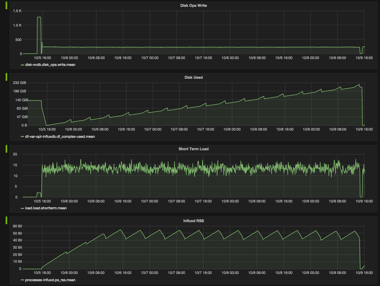
Disk writes, CPU usage, and storage consumption help operators recognize normal workload patterns and investigate sudden changes. Compare an observation with an appropriate baseline, such as the same hour on similar weekdays.
Health monitoring - how does a physiological signal vary over time?
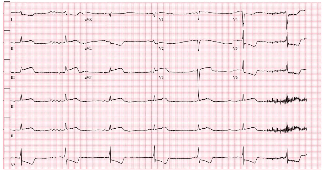
An electrocardiogram records electrical activity over time. Signal analysis can characterize the timing and shape of repeating patterns. Clinical interpretation requires the appropriate medical context and expertise.
Finance - how does a price series behave?
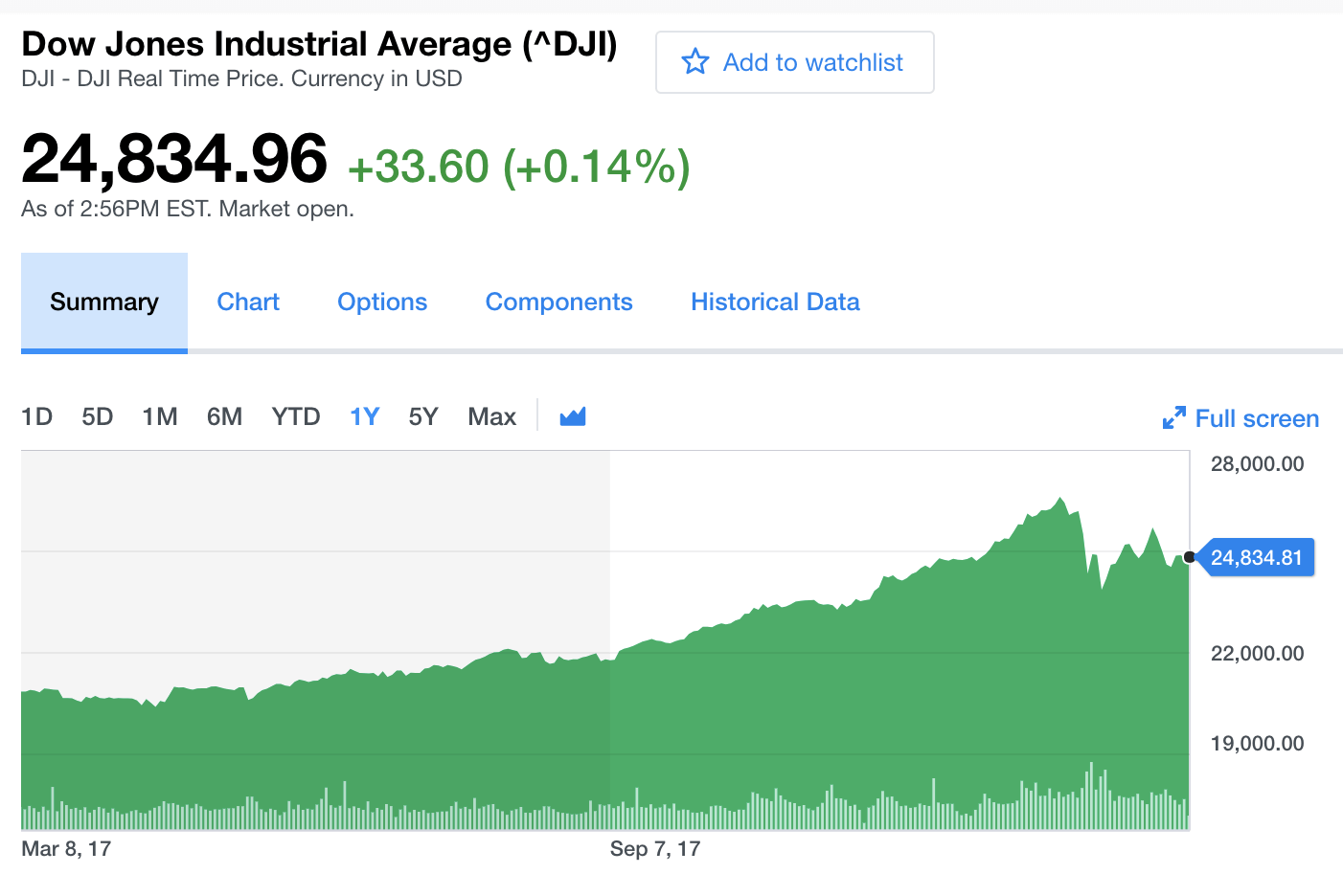
Price histories show changes, volatility, and periods of unusual movement. A historical chart provides evidence about observed behavior; it does not guarantee future prices.
Logs and traces - when did an operational problem occur?
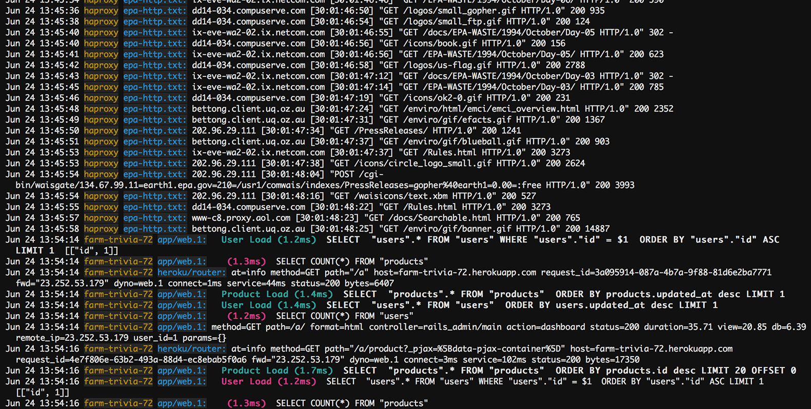
Logs record timestamped events and contextual messages. Counting errors by minute turns an irregular event stream into a regular series that can be compared with deployment times or traffic levels. Not every executable produces a log; logging depends on the application’s configuration.
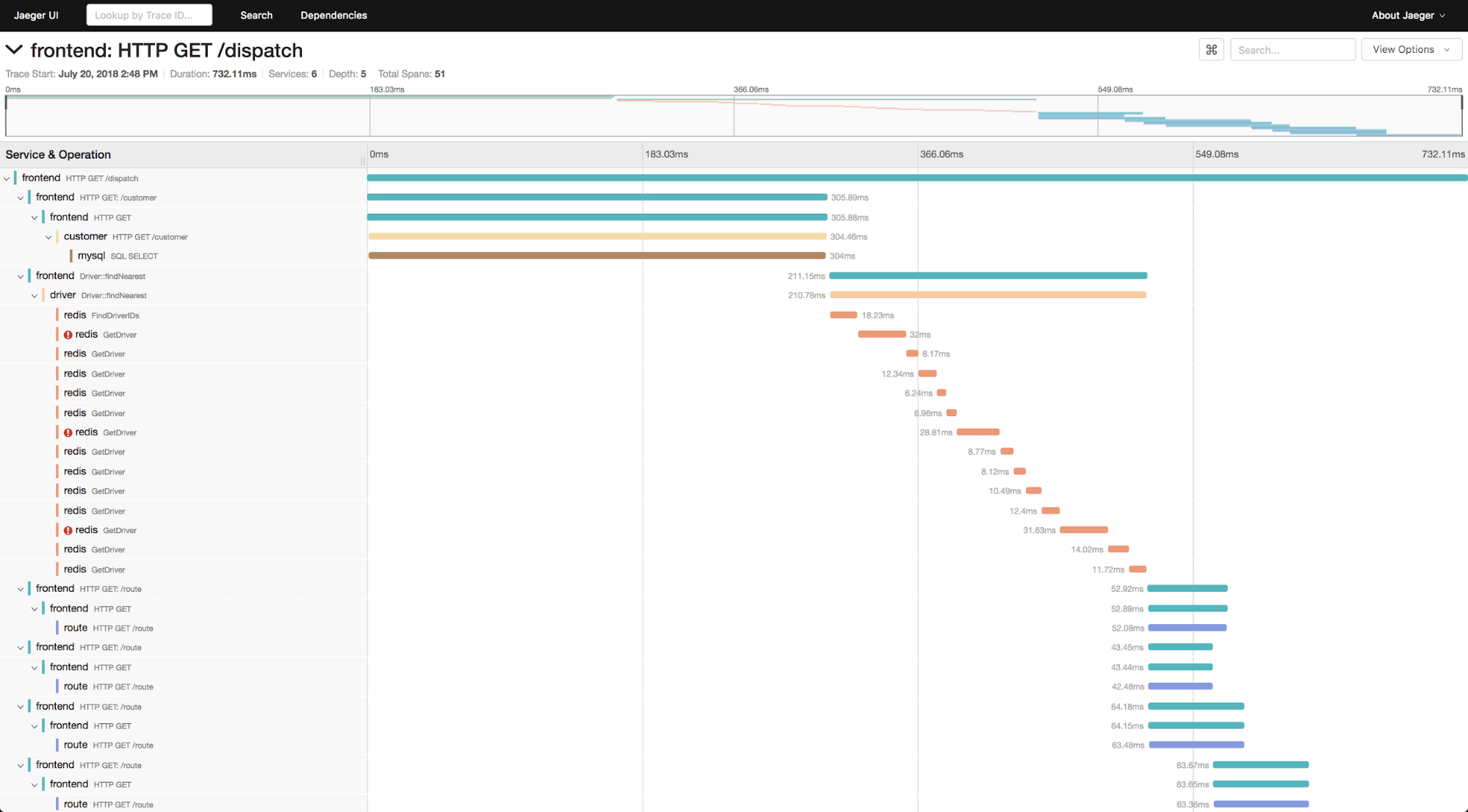
Distributed traces connect spans representing operations in a request. Span start times and durations help identify where a request spent time; aggregating request counts or durations over time supports time series analysis.
How can InfluxDB support time series analysis?
InfluxDB 3 Core stores timestamped measurements and supports querying them with SQL. Time-based aggregation helps prepare a series for visualization, comparison, and further analysis. See the SQL query guide for supported query patterns.
Example - compare hourly CPU usage
Assume a table named cpu_usage contains a timestamp column time, a host identifier host, and a numeric field cpu_percent. The following query returns an hourly average and maximum for one host over three days of available data.
SELECT
  DATE_BIN(
    INTERVAL '1 hour',
    time,
    '2026-09-01T00:00:00Z'::TIMESTAMP
  ) AS hour,
  host,
  AVG(cpu_percent) AS avg_cpu_percent,
  MAX(cpu_percent) AS max_cpu_percent
FROM cpu_usage
WHERE host = 'web-01'
  AND time >= '2026-09-01T00:00:00Z'::TIMESTAMP
  AND time < '2026-09-04T00:00:00Z'::TIMESTAMP
GROUP BY 1, host
ORDER BY hour, host;
The DATE_BIN reference documents the interval, timestamp, and origin arguments. Adjust the table, columns, host, and date range to match your data. For setup and ingestion, follow the Core getting-started guide and write guide.
This illustrative subset of hourly averages is invented to explain the analysis; it is not customer data or measured query output.
| UTC hour | Day 1: CPU usage (%) | Day 2: CPU usage (%) | Day 3: CPU usage (%) |
|---|---|---|---|
| 09:00 | 30 | 34 | 38 |
| 13:00 | 50 | 54 | 95 |
| 17:00 | 35 | 39 | 43 |
- Possible trend: the selected 09:00 and 17:00 values rise across the three days. A longer history would be needed to establish a sustained trend.
- Possible daily pattern: 13:00 is the busiest selected hour each day. More repeated cycles would help confirm seasonality.
- An observation to investigate: Day 3 reaches 95% at 13:00, compared with 50% and 54% on the preceding days. Check traffic, deployments, and host conditions before calling it a fault.
Keep raw values and compare hourly maxima as well as averages when short spikes matter. An hour with no observations is missing, not automatically zero. A forecasting task would then fit and evaluate a model using a suitable statistical tool or analysis workflow; this aggregation query itself does not produce a forecast.
Historical case study - Robinhood anomaly detection
Robinhood describes using InfluxDB with Faust and Kafka for monitoring and alerting. Robinhood compared aggregated observations with historical mean and standard-deviation bounds.
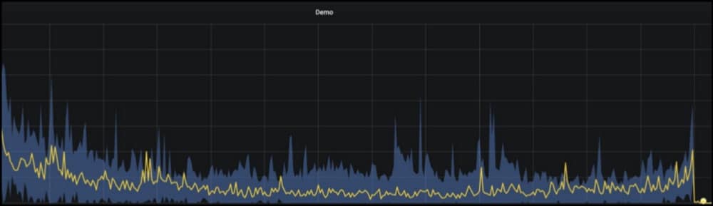
A fixed threshold can generate alerts during an expected trend or recurring peak. A baseline that accounts for relevant historical behavior can give those observations more context.

For a normal distribution, approximately 99.73% of values lie within three standard deviations of the mean, leaving approximately 0.27% outside the interval across both tails. That percentage depends on the distributional assumption and is not a guarantee for arbitrary telemetry.

A standard-deviation threshold does not automatically follow a trend. Its behavior depends on how the baseline is estimated and updated; seasonality, changing variance, and departures from normality require further consideration.
For another example, the Epsilon3 case study explains its use of InfluxDB to support real-time operations during aerospace missions.
What common mistakes should you avoid?
- Confusing missing data with zero: A missing sensor reading and an actual zero value mean different things. Investigate gaps and document any interpolation or other filling method.
- Combining unrelated series: Group by relevant host, sensor, location, or other identifiers. Combining entities can hide local anomalies.
- Aggregating too aggressively: A daily average can conceal a brief outage. Select a resolution that matches the decision and preserve finer observations when needed.
- Using future information during evaluation: Fit preprocessing and model choices using training data. When forecasting, avoid random shuffling and using future observations to fill past gaps or construct features.
- Treating correlation as causation: Two series may move together because of a shared trend or seasonal pattern. Investigate alternative explanations.
- Assuming every unusual point is an error: A spike may be a real event, a measurement problem, or an expected change. Check context before removing it.
- Assuming time series data must be immutable: New observations are often appended, but late arrivals and corrections can occur. Record correction and deduplication rules.
- Choosing a complex model without a baseline: Compare forecasting results with a simple alternative and report uncertainty. Revalidate when the underlying process changes.
To continue learning, explore time series visualization and InfluxDB University.