When You Want Holt-Winters Instead of Machine Learning

By Anais Dotis-Georgiou / Product, Use Cases, Developer
Feb 21, 2019

Machine Learning (ML) gets a lot of hype, but its classical predecessors are still immensely powerful, especially in the time-series space. Error, Trend, Seasonality Forecast (ETS), Autoregressive Integrated Moving Average (ARIMA) and Holt-Winters are three classical methods that are not only incredibly popular but are also excellent time-series predictors.

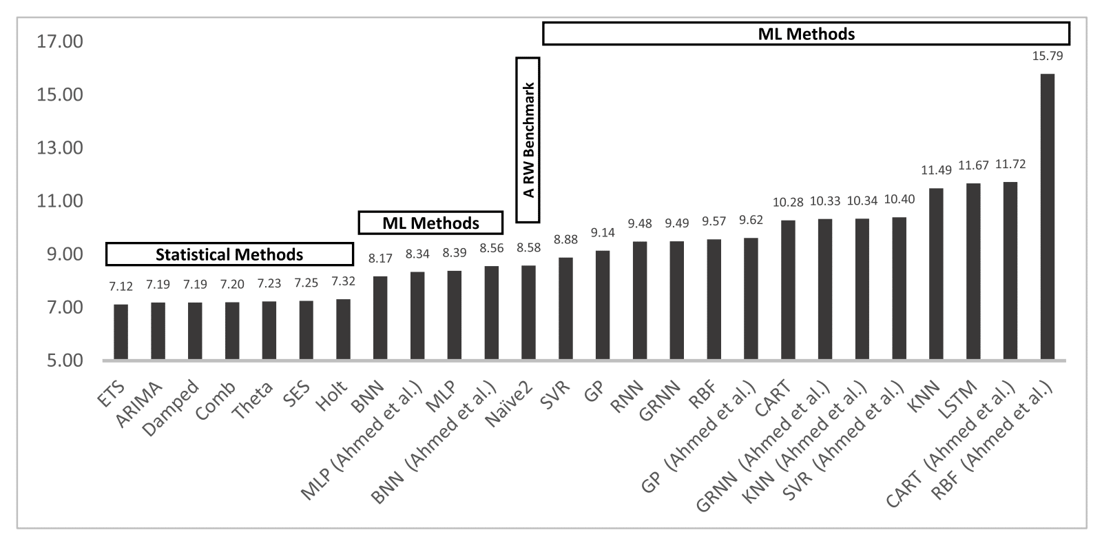
In fact, according to Statistical and Machine Learning forecasting methods: Concerns and ways forward, ETS outperforms several other ML methods including Long Short Term Memory (LSTM) and Recurrent Neural Networks (RNN) in One-Step Forecasting. Actually, all of the statistical methods have a lower prediction error than the ML methods do.

My hope is that after finishing this three-part blog post series, you’ll have a strong conceptual and mathematical understanding of how Holt-Winters works. I focus on Holt-Winters for three reasons. First, Holt-Winters or Triple Exponential Smoothing is a sibling of ETS. If you understand Holt-Winters, then you will easily be able to understand the most powerful prediction method for time series data (among the methods above). Secondly, you can use Holt-Winters out of the box with InfluxDB. Finally, the InfluxData community has requested an explanation of Holt-Winters in this Github issue 459. Luckily for us, Holt-Winters is fairly simple, and applying it with InfluxDB is even easier.

In this current piece, Part One of this blog series, I’ll show you:

1. When to use Holt-Winters;
2. How Single Exponential Smoothing works;
3. A conceptual overview of optimization for Single Exponential Smoothing;
4. Extra: The proof for optimization of Residual Sum of Squares (RSS) for Linear Regression.

In Part Two, I’ll show you:

1. How Single Exponential Smoothing relates to Triple Exponential Smoothing/Holt-Winters;
2. How RSS relates to Root Mean Square Error (RMSE);
3. How RMSE is optimized for Holt-Winters using the Nelder-Mead method.

In Part Three, I’ll show you:

1. How you can use InfluxDB's built-in Multiplicative Holt-Winters function to generate predictions on your time-series data;
2. A list of learning resources.

When to use Holt-Winters

Before you select any prediction method, you need to evaluate the characteristics of your dataset. To determine whether your time series data a good candidate for Holt-Winters or not, you need to make sure that your data:

• Isn't stochastic. If it is random, then it's actually a good candidate for Single Exponential Smoothing;
• Has a trend;
• Has seasonality. In other words, your data has patterns at regular intervals. For example, if you were monitoring traffic data, you would see a spike in the middle of the day and a decrease in activity during the night. In this case, your seasonal period might be one day.

How Single Exponential Smoothing works

Before we dive into Holt-Winters or Triple Exponential Smoothing, I’ll explain how Single Exponential Smoothing works. Single Exponential Smoothing (SES) is the simplest exponential smoothing method (exponential smoothing is just a technique for smoothing time-series data where exponentially decreasing weights are assigned to past observations). It is built upon the Naïve Method. With this method, the forecasted value is equal to the last observed value,

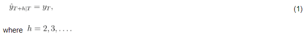
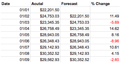
Hard to believe that Naïve would want to be credited with such a simple model, but it turns out it’s quite good at predicting financial data. Also, taking the percent difference between the actual and predicted values can be a good way to uncover seasonality.

Single Exponential Smoothing (SES) agrees with the Naïve method in that future values can be predicted from the looking at the past, but it goes a bit further to say that what has happened most recently will have the largest impact on what will happen next. A forecast from SES is just an exponential weighted average.

where 0 ? ? ? 1 is the smoothing parameter. A smoothing parameter relates the previous smoothed statistic to the current observation and is used to produce a weighted average of the two. There are a variety of methods to determine the best smoothing parameter. However, minimizing the RSS (residual sum of squared errors) is probably the most popular. (We will cover this in Part Two.) It’s also worth noticing that if alpha = 1, then SES reduces back to the Naïve Method.

The following table shows the weights for each observation for an alpha = 0.2. The weights decrease exponentially, thereby lending most recent observation the largest impact on the prediction.

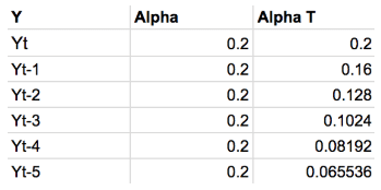
This table shows the weights attached to observations for an alpha = 0.2. Notice how the sum of these weights approaches 1. More simply, this guarantees that your prediction is on the same scale as your observations. If the sum of the weights was equal to 1.5, your output would be 50 percent greater than your observations. The sum of the weights converging to 1 is a geometric convergence.

Mathematicians love to rewrite formulas. Next, we’ll take a look at how we get the Component form of SES because it is the same form that is most commonly used to express Holt-Winters.

We simply use l_(t) to denote the smoothing equation. Meanwhile, l_(t-1) denotes the previous forecast. In this way, we get to encapsulate the iterative nature of Eq. (2) concisely.

However, there are two points that we have not addressed. The first is that we don’t know how to find alpha. Secondly, you probably made an astute observation about Eq. (3). It’s iterative, so what happens at the beginning, at time 1, when we have l_nought? The short answer is that we minimize the RRS (residual sum of squared errors) to find both alpha and l_nought. The long answer is in in the next section.

A conceptual overview of optimization for Single Exponential Smoothing

In this section, I explain how to find the regression line. In doing so, you end up having a great math analogy that helps you understand how alpha and l_nought are calculated for SES. In this section, I merely set up the steps conceptually. Following this section, you can find the proof for linear regression optimization by minimizing the Residual Sum of Squared Errors (RSS).

Let’s take a look at the smoothing equation at time 1:

Notice how it looks a lot like the point-slope form of a line:

The optimization of Eq. (4) is what you would actually optimize if you wanted to find the smoothing parameters for SES. However, for this section, we substitute Eq. (5) for Eq. (4) for simplification purposes. We then find the optimal m and b by minimizing the Sum of Squared Errors (RSS). Once we have found the optimal m and b, we have found the regression line. These same steps are used to find the smoothing parameters for Holt-Winters. The only difference is that minimizing the RSS to the regression line is only a 3-D optimization problem and that the proof is 90 percent algebra while finding the smoothing parameters for Holt-Winters is multi-dimensional and requires a lot of differential equations.

In order to understand how to minimize RSS, you need to know what it is. RSS is defined by:

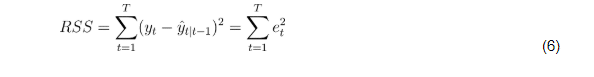
It’s a measure of error between our data points and the line of best fit.

Let’s take a look at our data:

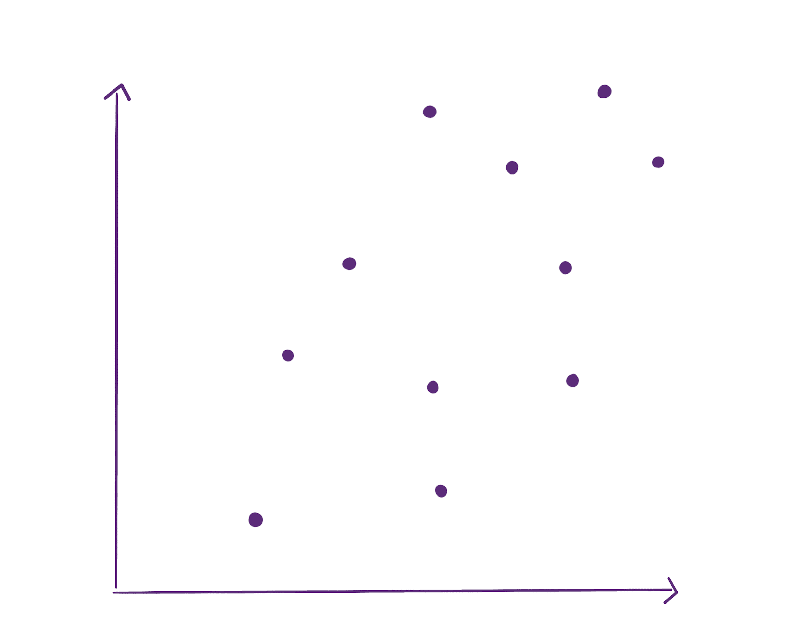
It’s random, but we can find a regression line or line of best fit. To do so, we draw a line and find the RSS for that line.

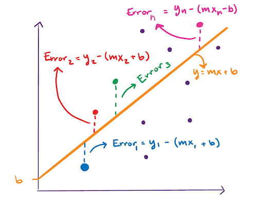
We find the RSS by taking the sum of all of these errors squared. Now imagine that we draw a bunch of different lines and calculate the RSS hundreds of times. The RSS can now be visualized in 3-D as a sort of bowl, where the value of the RSS depends on the line we draw. The line we draw is defined by its slope, m, and y-intercept, b.

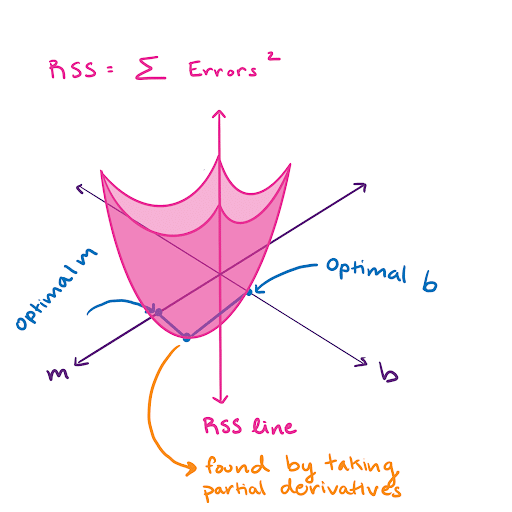
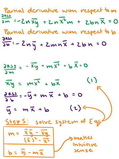
At the very bottom of this bowl is the optimal slope. We take the partial derivative of the RSS and set it equal to 0. Then we solve for m and b. That’s all there is to it. Linear regression optimization is pretty simple. Finding the smoothing parameters for Single Exponential Smoothing is done in the same way.

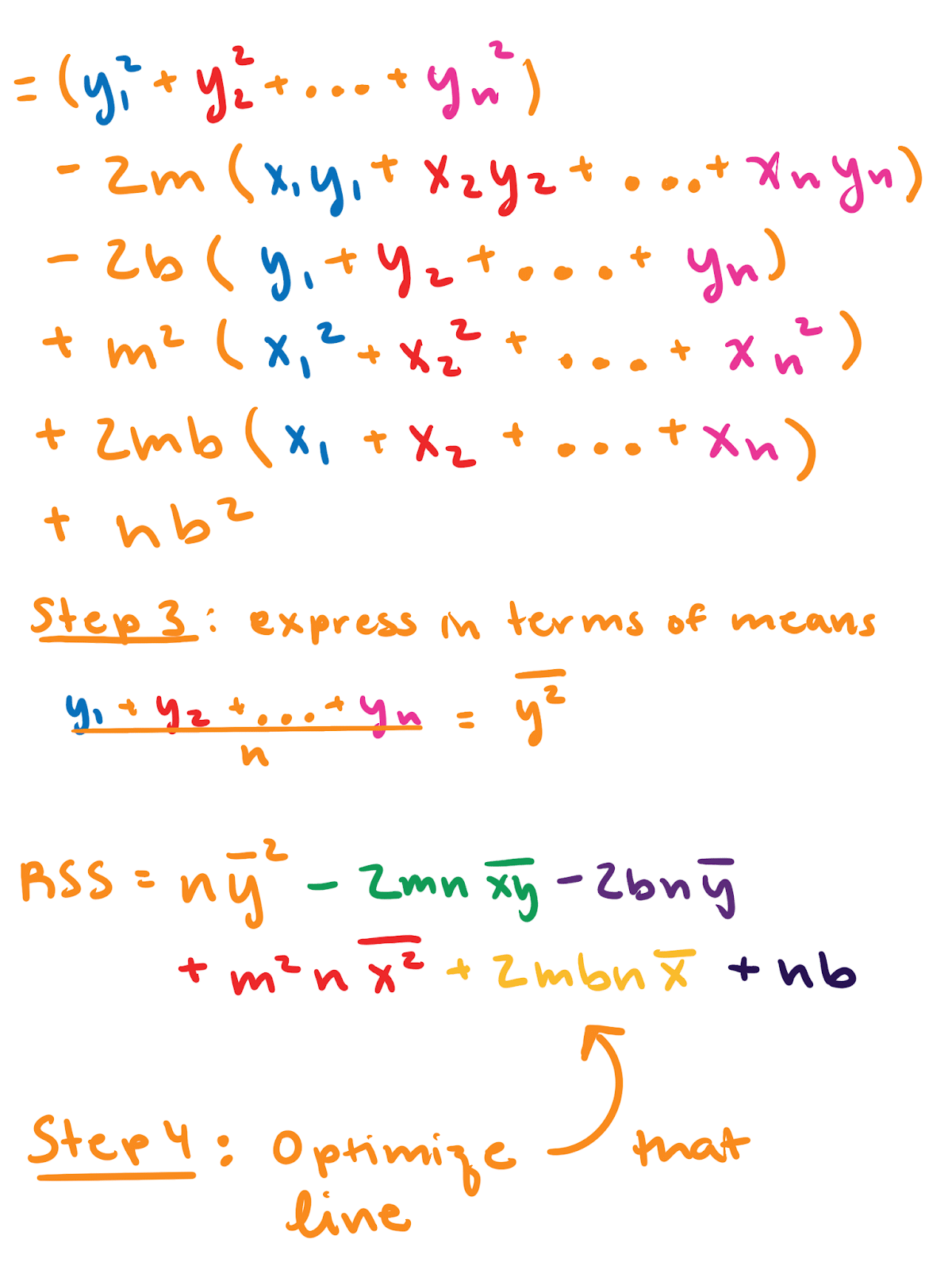
Extra: The proof for optimization of RSS for Linear Regression

If you’re like me, you need to see some math to feel satisfied. “The proof is in the mathing,” as I said in that one blog. If you’re already convinced or you don’t like math, skip this section. It’s colored to match the graph in the “A conceptual overview of optimization for Single Exponential Smoothing” portion of this blog.

Thanks for sticking with me and congratulations on making it this far. I hope this tutorial helps get you started on your forecasting journey. If you have any questions, please post them on the community site or tweet us @InfluxDB. You’ve deserved this well-earned brain break: