How To: Building Flux Queries in Chronograf
By
David G. Simmons
updated December 14, 2025
Product
Developer
Navigate to:
As you all may or may not know (and if you don’t, you haven’t been reading my posts!), I’ve built an embedded IoT gateway proof of concept device that runs (of course) InfluxDBreally the entire TICK Stackand collects data from connected Bluetooth, WiFi and LoRa sensors.
The latest releases of InfluxDB and Chronograf are now available, and with each of these, comes the technical preview of Flux, the new query language for working with time series data. I thought it might be instructive to see how difficult it was going to be to convert the queries that I use to build my dashboard from InfluxQL to Flux and generally explore the language itself. So here goes.
The Dashboard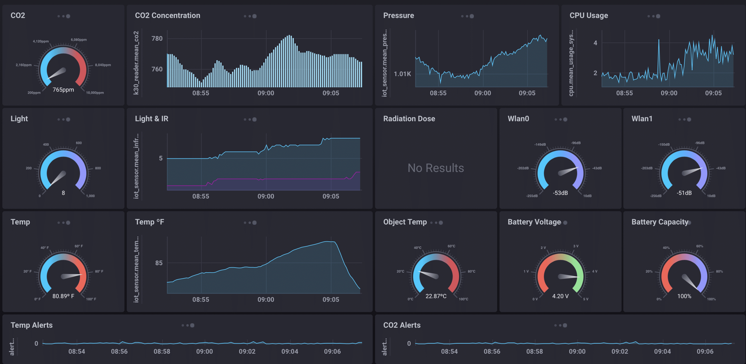
That’s all the sensor datawell, the radiation sensor is off-line right nowand how it looks on-screen. Each of those dashboard elements is created and updated via an InfluxQL query via Chronograf. So let’s look at some of the queries and what they look like in the Chronograf Dashboard Builder today. We’ll start with that CO2 reading at the upper left:

To be perfectly clear: I did not have to write that query. I simply started exploring the database, clicking on measurements, tags and values, and adjusting the settings until I got the visualization I was looking for. Easy enough.
So let’s try building that same query in using InfluxDB 1.7, Chronograf 1.7 and using the new Flux Builder along with the Schema Explorer:
Wow! That was easy!
It’s very, very similar. In the Flux example, we start with where we’re going to get the datathe ‘from bucket’and then give it the time interval, and finally filter by the measurement and field.
Next, we add the window(every: autoInterval) to the query. Flux’s window() function groups records based on a time value. Using the every: parameter along with autoInterval allows Chronograf to dynamically determine the size of the window based on the screen real-estate that is available for visualizing the results.
And here’s what the Flux query looks like in the end:
from ( bucket: "telegraf/autogen" )
   |> range(start: dashboardTime)
   |> filter (fn: (r) => r._measurement == "k30_reader" and (r_field == "co2" ))
   |> window (every: autoInterval)
Flux takes input tables, performs a function, and produces one or more output tables. So far, we’ve defined an input table. Now, we add the mean() aggregate function to get the mean CO2 reading within each window. Each window is returned as an output table. By adding the group() function with the none:true parameter, we remove the window partitions and combine the aggregates into a single output table.
The resulting query looks like this:
from(bucket: "telegraf/autogen")
  |> range(start: dashboardTime)
  |> filter(fn:(r =>r._measurement == "k30_reader" and (r._field == "co2"))
  |> window(every: autoInterval)
  |> mean()
  |> group(none:true)
The original query used the template variable :dashboardTime: to allow the user to adjust the time range of the query through the user interface controls provided within Chronograf without forcing them to re-adjust the query itself. This same functionality is supported within Flux too. The ScriptWizard drops this into the |> range filter by default.
Now we can visually compare the results by flipping back and forth between the InfluxQL and the Flux version of these queries to see that they indeed yield the same results!
What about FILL?
In the technical preview of Flux, the fill functionality hasn’t been implemented. We understand this is an important part of how to visualize sparse data and rest assured we are working to implement this in a future update.
