Part 5: How to Create an IoT Project with the TICK Stack on the Google Cloud Platform

By Todd Persen / Product, Use Cases
Mar 01, 2016

Part 5: Visualizing IoT Sensor Data with Chronograf

So far in the series, we’ve managed to set up InfluxDB and it is now receiving data from various temperature stations. While we can use the InfluxDB web application to query for data, it falls short when it comes to visualizing the same data via charts and dashboards. For e.g. an ability to continuously monitor the data and see it on a graph.

In this part of the tutorial, we are going to look at Chronograf. Chronograf is the “C” in the TICK stack and is used for visualization of InfluxDB data. We can use this tool to look at the temperature readings that have been reported via various stations.

Chronograf is a standalone application that you need to setup on a system. This could reside on premises or in the cloud or even running on your laptop, as we are going to see. As long as you configure it to point to the appropriate InfluxDB data and setup your graphs/dashboards, you can run it from anywhere. Below is a simple GIF that gives you an idea of the how the interface looks:

Setting up Chronograf

Download instructions for setting up Chronograf are straightforward. We are going to set Chronograf up on a Mac machine. Note that you can set it up on other platforms too like RedHat, Ubuntu, Debian, etc.

We used Homebrew, the package manager on the Mac to install Chronograf as shown below:

<span style="font-weight: 400;">$ brew install homebrew/binary/chronograf</span>

The installation proceeds and gives you instructions to start Chronograf once the process is complete.

==> Tapping homebrew/binary
Cloning into '/usr/local/Library/Taps/homebrew/homebrew-binary'...
remote: Counting objects: 26, done.
remote: Compressing objects: 100% (26/26), done.
remote: Total 26 (delta 1), reused 4 (delta 0), pack-reused 0
Unpacking objects: 100% (26/26), done.
Checking connectivity... done.
Tapped 22 formulae (71 files, 49.5K)
==> Installing chronograf from homebrew/binary
==> Downloading https://s3.amazonaws.com/get.influxdb.org/chronograf/chronograf-
######################################################################## 100.0%
==> Caveats
To run Chronograf manually, you can specify the configuration file on the command line:

 chronograf -config=/usr/local/etc/chronograf.toml

To have launchd start homebrew/binary/chronograf at login:

 ln -sfv /usr/local/opt/chronograf/*.plist ~/Library/LaunchAgents

Then to load homebrew/binary/chronograf now:

 launchctl load ~/Library/LaunchAgents/homebrew.mxcl.chronograf.plist

==> Summary
?  /usr/local/Cellar/chronograf/64: 3 files, 14.0M, built in 38 seconds

$

Starting Chronograf

We start Chronograf next via the -config option as shown below. The chronograf.toml files points to various configuration settings and we can go ahead with the default values for now.

$ chronograf -config=/usr/local/etc/chronograf.toml
[chronograf] 2016/01/12 20:17:06 Starting Chronograf (version 0.4.0)
[chronograf] 2016/01/12 20:17:06 Server binding to http://127.0.0.1:10000
[chronograf] 2016/01/12 20:17:06 Reporting anonymous usage statistics

The next step is to launch the Chronograf Web Application. As pointed out in the console output above, the server has been launched on port 10000. Since we want to run the web application locally itself, we simply launch a browser and visit http://localhost:10000.

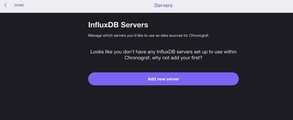
This brings up the UI as shown below and it is along expected lines i.e. we have not defined any InfluxDB Servers as of yet in the Chronograf application.

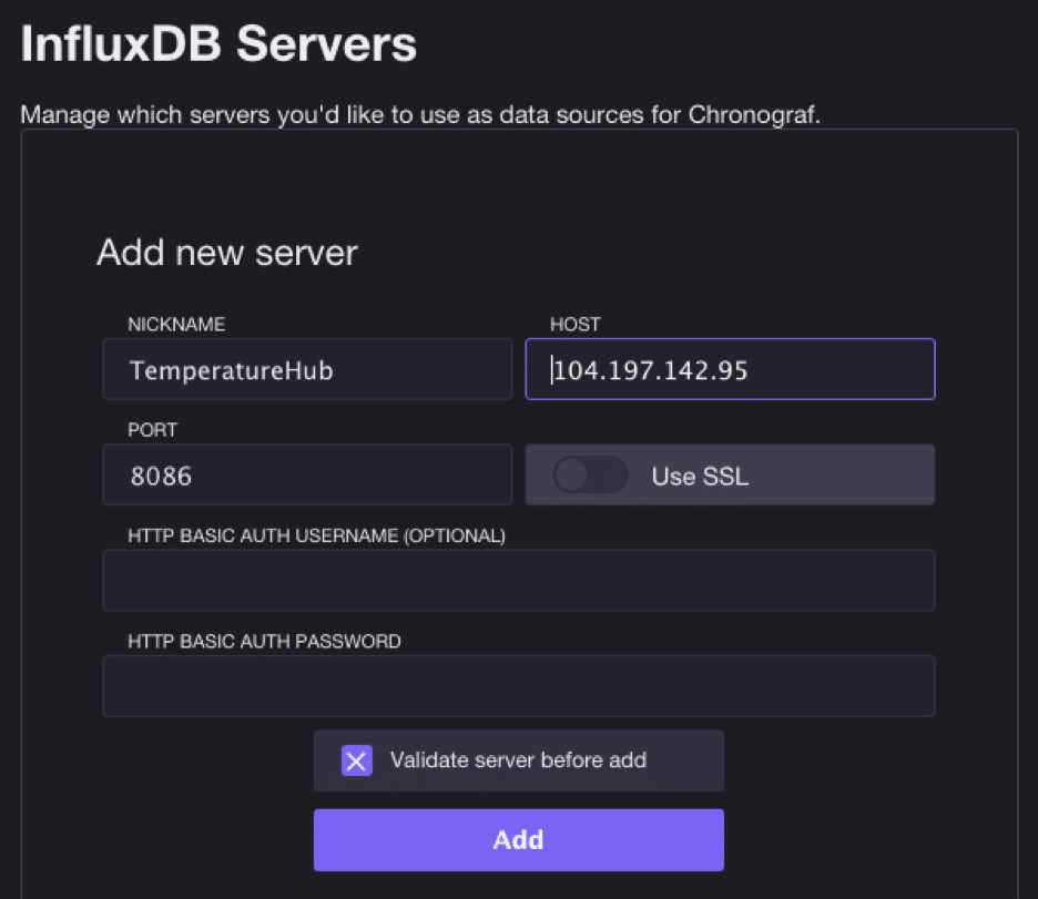
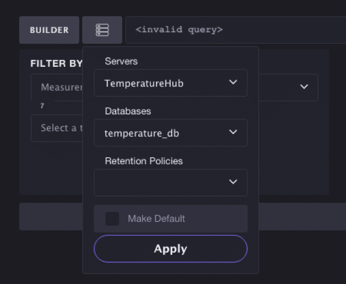
Click on Add new server to add an InfluxDB database instance. This will bring up the form as shown below and we populate the values as follows:

• Nickname : You can give any name in here. We have named it TemperatureHub
• Host : This is the IP Address of the Influx DB instance. Since we have hosted it on the Google Compute Engine instance, this is the Public IP Address of the Compute Engine instance, that we have been using all the while.
• Port : The Chronograf application will communicate with the InfluxDB instance via the API that is running on port 8086 of the InfluxDB instance. We had opened up the firewall on the InfluxDB Compute Engine instance to allow traffic on port 8086. We enter 8086 as the port number value here.
• Click on Add.

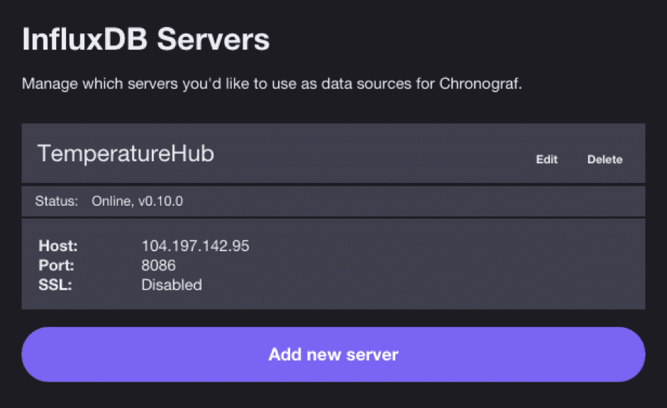
This will add the InfluxDB Server to Chronograf and we can click on Done.

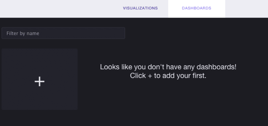
This will then lead to a screen as shown below where you can see both Visualizations and Dashboards shown as options. Both of these tab views are empty, since we have not yet defined any of them.

Think of Dashboards as a container for all your graphs. For e.g. We will define a Dashboard for e.g. that can show up the temperature readings from both Station S1 and Station S2. We will define both of the Station temperature readings as Graph and add them to the Dashboard so that we can see it together in a single dashboard.

Let’s create our dashboard then.

Creating our first Dashboard

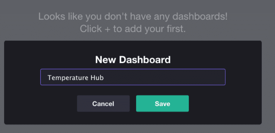
Click on the DASHBOARDS tab option as shown below.

Then click on + sign to add a new Dashboard. This brings up the screen below and we give a name Temperature Hub to our dashboard.

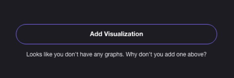
Click on Save to continue. As mentioned below, a dashboard is really a container for your graphs and hence you will see a message as shown below.

Click on Add Visualization to add a graph. We want to define Graphs for visualizing the temperature sensor values from both Station 1 and Station 2. So, let’s define the graph for Station 1 first as shown below. We give it a name Station 1 and click on Save.

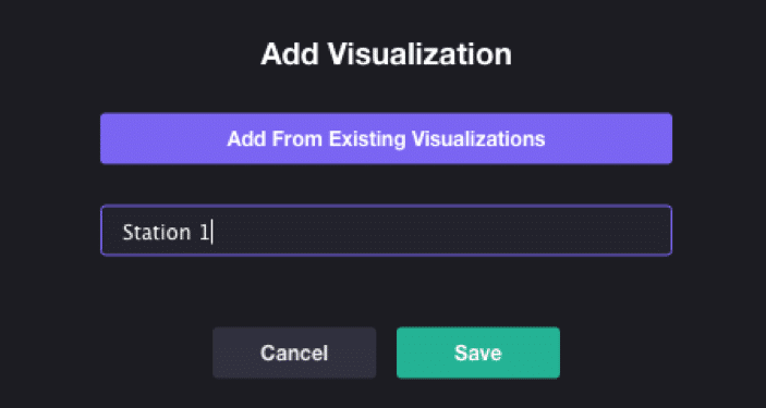Note: Visualizations are reusable in other Dashboards. Notice how the above screen allows us to select from Existing Visualizations too.

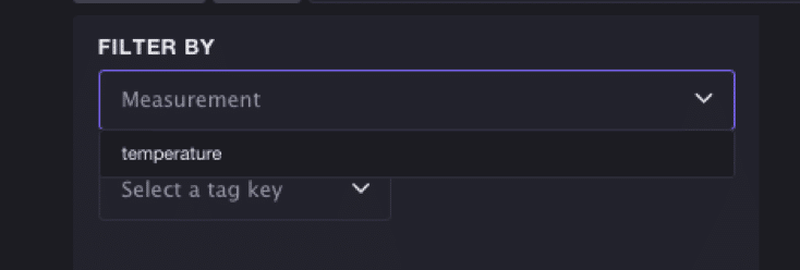
Things are pretty intuitive from here on. The steps are:

Select the correct database (temperature_db) from our InfluxDB instance.

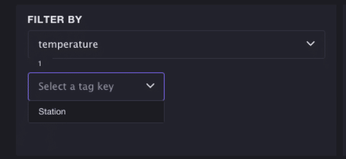
Select the measure (temperature) Add filters for the Station Name (use the tag key Station and value ‘S1’) 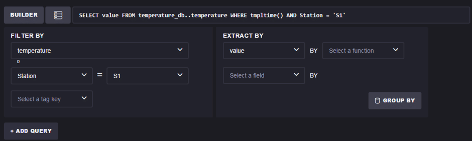Notice that the query that has been selected is shown for clarity below:

SELECT value FROM temperature_db..temperature WHERE tmpltime() AND Station = 'S1'

The query is modifiable and keep that in mind, just in case you find that you do have data but it is not displaying on the graph. You can tweak this as per your requirements.

We created another graph named Station 2 and added similar configuration values, except that the Station = 'S2'.

Chronograf in Action

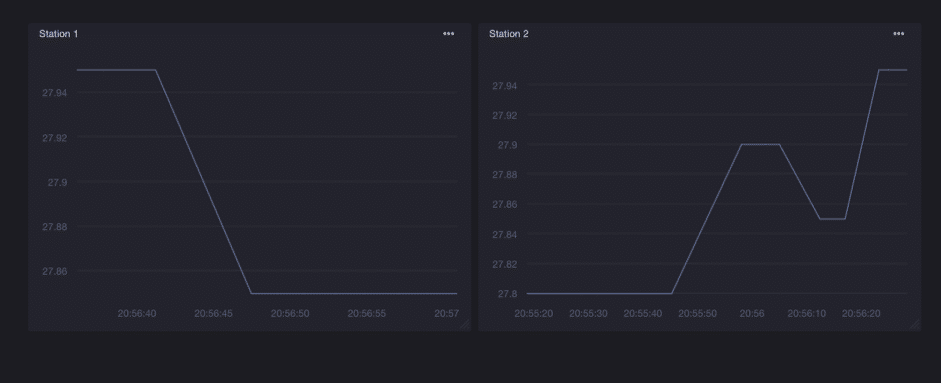
The Dashboard springs to life almost immediately as the values come in. A sample run is shown below for values being received from our 2 temperature stations : S1 and S2.

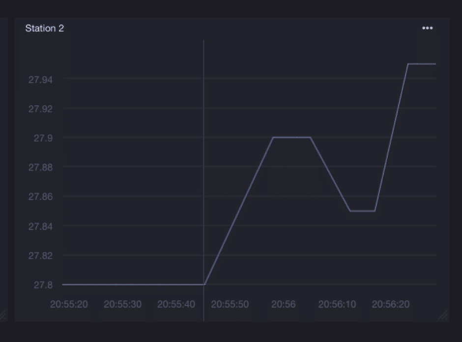
And here is a zoom in for Station 2 dashboard.

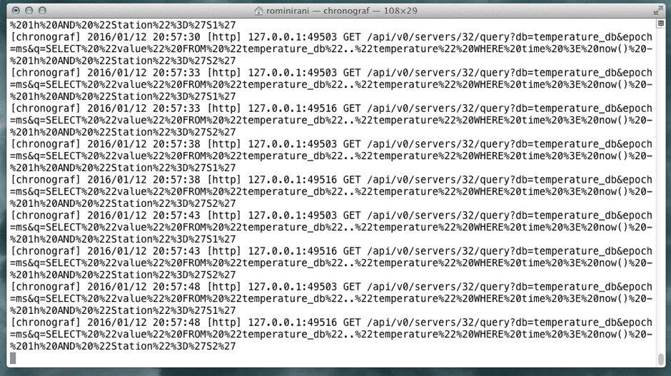
If I switch to the Chronograf Server console, I can see that it is pretty busy invoking the REST APIs to fetch the data.

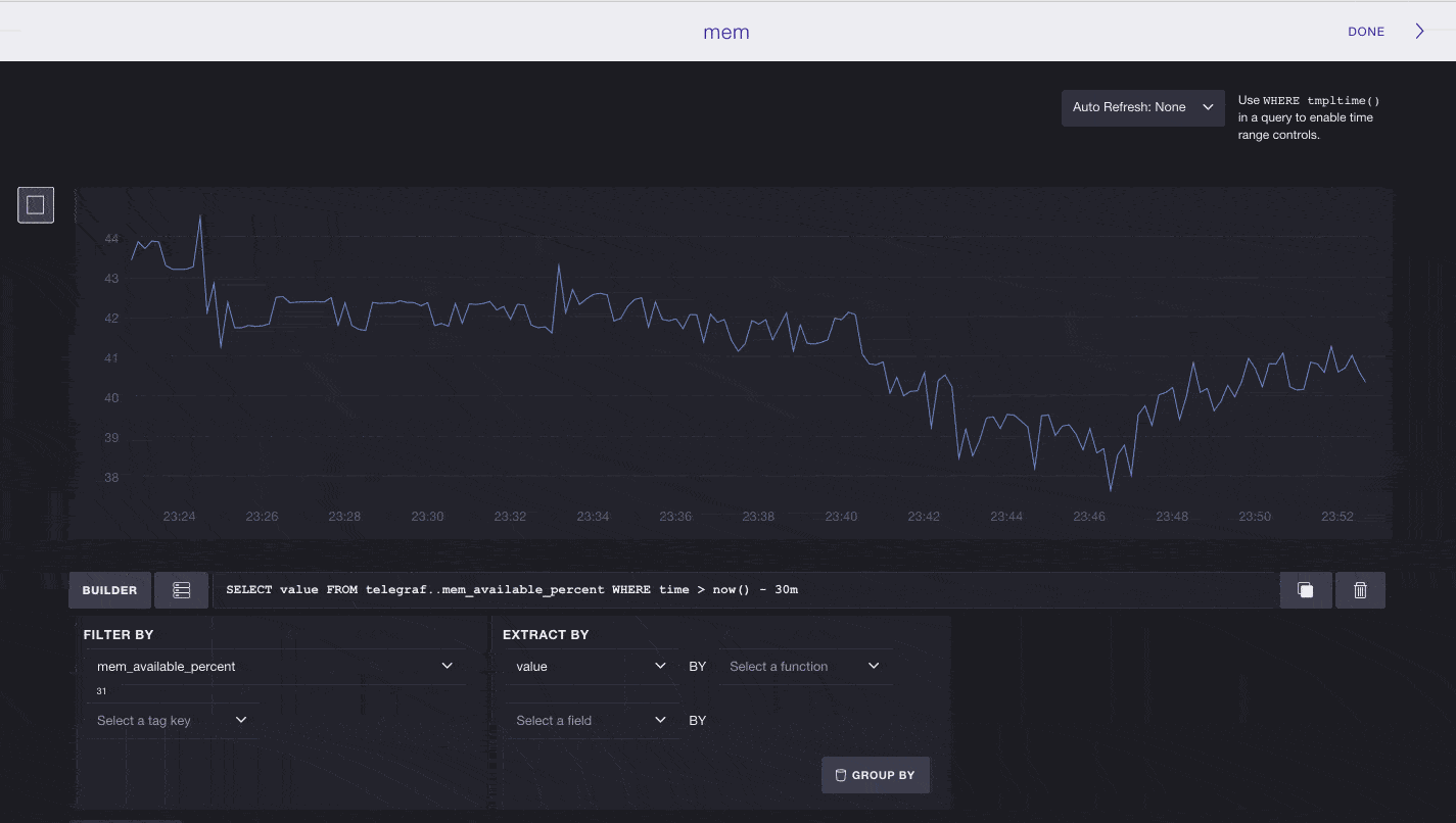
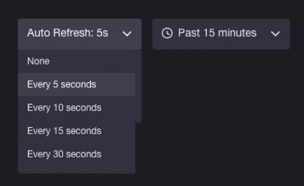
Configuring Auto Refresh and Time Filter for data

The Chronograf web application refresh interval (to update the UI) is completely configurable via the Settings as shown below. In addition, you also notice that the default filter for data was records that have been received in the last 15 minutes. That setting is configurable too and is the drop down next to Auto Refresh in the screen below.

This completes our first look at setting up Chronograf, a great module in the TICK stack to visualize your time series database.

What's next?

• In part six, we will explore how to use Kapacitor to setup alerts to Slack depending on certain threshold values we see in the data. Follow us on Twitter@influxdb to catch the next blog in this series.
• Looking to level up your InfluxDB knowledge? Check out our economically priced virtual and public trainings.