InfluxDB: How to Do Joins, Math across Measurements

By Anais Dotis-Georgiou / Product, Use Cases, Developer
Dec 13, 2018

If you’re part of the InfluxData community, then you’ve probably wanted to perform math across measurements at some point. You did some googling and stumbled on this GitHub issue 3552 and shed a small tear. Well, today I get to be the bearer of good news. InfluxData has released the technical preview of Flux, the new query language and engine for time series data, and with it comes the ability to perform math across measurements.

In this blog, I share two examples of how to perform math across measurements:

1. How to calculate the batch size of lines written to the database per request. Following this example is the fastest way to explore math across measurements. You can simply get the sandbox up and running, and copy and paste the code to try it for yourself.
2. How to "monitor" the efficiency of a heat exchanger over time. You can find the dataset and Flux query for this part are located in this repo.

To learn about all the features of Flux, please look at the specification and the companion documentation.

How to calculate the batch size of lines written to the database per request

After you clone the sandbox and run ./sandbox up, you will have the entire TICK Stack running in a containerized fashion. The “telegraf” database contains several metrics gathered from your local machine. To calculate the batch size of the metrics being gathered and written to InfluxDB, we need to find the number of lines written to the database over time and divide that value by the number of write requests during that same time period.

First, filter the data to isolate the number of write requests made and lines written. Store that data in two tables, “httpd” and “write”, respectively.

httpd = from(bucket:"telegraf/autogen")
|> range(start: dashboardTime)
|> filter(fn:(r) => r._measurement == "influxdb_httpd" and r._field == "writeReq")

write = from(bucket:"telegraf/autogen")
|> range(start: dashboardTime)
|> filter(fn:(r) => r._measurement == "influxdb_write" and r._field == "pointReq")

Next, join the two tables. The Join defaults to a left join. Finally, we use the Map function to divide the two values and calculate the mean batch size over the Dashboard time (-5m).

avg_batch_size = join(tables:{httpd:httpd, write:write}, on:["_time"])
|> map(fn:(r) => ({
_value: r._value_write / r._value_httpd}))
|> mean()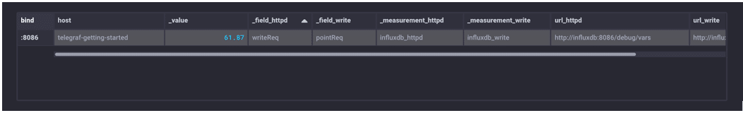

I change my visualization type to “Table” because my Flux script only returns one value. We can see that the average batch size over the last 5 minutes is ~62 lines/write.

Side note: While this query is easy, it’s rather inefficient. It is just for demonstration purposes. If you wanted to look at the average batch size over a longer time range, you might want to 1) window the httpd table and write table and  2) calculate the mean and max, respectively. Doing something like that will allow you to aggregate the data before performing math across measurements, which will be faster and more efficient.

How to "monitor" the efficiency of a heat exchanger over time

For this example, I decided to imagine that I am an operator at a chemical plant, and I need to monitor the temperatures of a counter-current heat exchanger. I collect temperatures of the cold (TC) and hot (TH) streams from four different temperature sensors. There are two inlet (Tc2, Th1) sensors and two outlet (Tc1, Th2) sensors at positions x1 and x2 respectively.

After making some assumptions, I can calculate the efficiency of heat transfer with this formula:

I collect temperature reading from each sensor at 2 different times for a total of 8 points. This dataset is small for demonstration purposes. My database is structured like this:

Since the temperature readings are stored in different measurements, again I apply Join and Map to calculate the efficiency. I am using the Flux editor and Table view in Chronograf to visualize all of the results.

First, I want to gather the temperature readings for each sensor. I start with Th1. I need to prepare the data. I drop the “_start” and “_stop” columns because I’m not performing any group by’s or windowing. I can drop the “_measurement” and “_field” because they are the same for all of my data. Finally, I am not interested in performing any analysis based on the “position”, so I can drop this as well. I will just be performing math across values on identical timestamps, so I keep the “_time” column.

Th1 = from(bucket: "sensors")
  |> range(start: dashboardTime)
  |> filter(fn: (r) => r._measurement == "Th1" and r._field == "temperature")
  |> drop(columns:["_start", "_stop", "_measurement", "position", "_field"])

Now I can apply the same query to Th2.

Th2 = from(bucket: "sensors")
  |> range(start: dashboardTime)
  |> filter(fn: (r) => r._measurement == "Th2" and r._field == "temperature")
  |> drop(columns:["_start", "_stop", "_measurement", "position", "_field"])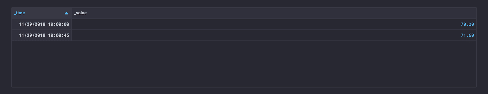

Next, I join the two tables.

TH = join(tables: {Th1: Th1, Th2: Th2}, on: ["_time"])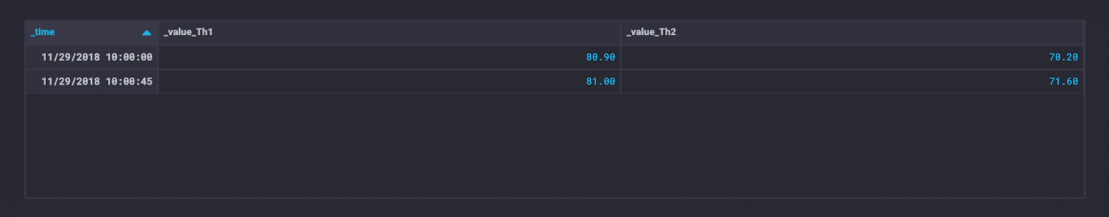

The Join defaults to a left join. tables: {Th1: Th1, Th2: Th2} allows you to specify the naming of your suffixes (equivalent to “rsuffix/lsuffix” in Pandas or the “table.id” syntax in SQL).

I apply this logic to the cold stream as well:

TC = join(tables: {Tc1: Tc1, Tc2: Tc2}, on: ["_time"])

Next, I join TC with TH.

join(tables: {TC: TC, TH: TH}, on: ["_time"])

Finally, I can use Map to calculate the efficiency across all of the measurements. This is what the code looks like all together:

Th1 = from(bucket: "sensors")
  |> range(start: dashboardTime)
  |> filter(fn: (r) => r._measurement == "Th1" and  r._field == "temperature")
  |> drop(columns:["_start", "_stop", "_measurement", "position", "_field"])

 Th2 = from(bucket: "sensors")
  |> range(start: dashboardTime)
  |> filter(fn: (r) => r._measurement == "Th2" and r. _field == "temperature")
  |> drop(columns:["_start", "_stop", "_measurement", "position", "_field"])

TH = join(tables: {Th1: Th1, Th2: Th2}, on: ["_time"])

Tc1 = from(bucket: "sensors")
  |> range(start: dashboardTime)
  |> filter(fn: (r) => r._measurement == "Tc1" and r._field == "temperature")
  |> drop(columns:["_start", "_stop", "_measurement", "position", "_field"])

Tc2 = from(bucket: "sensors")
  |> range(start: dashboardTime)
  |> filter(fn: (r) => r._measurement == "Tc2" and r._field == "temperature")
  |> drop(columns:["_start", "_stop", "_measurement", "position", "_field"])

 TCTH = join(tables: {Tc1: Tc1, Tc2: Tc2}, on: ["_time"]])
 join(tables: {TC: TC, TH: TH}, on: ["_time"])
|> map(fn: (r) => (r._value_Tc2 - r._value_Tc1)/(r._value_Th1 - r._value_Th2))
|> yield(name: "efficiency")

I can see that the heat transfer efficiency has decreased over time. This is a really simple example of the power of Flux, but it has my imagination running wild. Could I build a monitoring and alerting tool similar to DeltaV Alarm Management solutions with just the OSS? Probably not, but I can dream of someone who might.

If you’re like me and find contextualization and comparison useful, I recommend reading my upcoming UX review. In that review, I compare Flux Joins against Pandas Joins. Flux has some peculiarities. The most glaring one for me is the |>, pipe forward. At first, I disliked it. I almost never use pipes and my pinky finger whined at the thought of having to learn a new stroke. Now, I find that they greatly increase readability. Every pipe forward returns a result. Reading Flux queries feels like reading bullet points.