By Nga Tran / Andrew Lamb / Developer
Mar 18, 2024

This post explains how databases optimize queries, which can result in queries running hundreds of times faster. While we focus on one specific query type that is important to InfluxDB 3.0, the optimization process we describe is the same for any database.

Optimizing a query is like playing with Lego

You can come up with different structures when playing with the same set of Lego pieces, as shown in Figure 1. While you often use the same basic bricks to build whatever structure you want, there are times when you need a different type of shape (e.g., tiny star) for a specific project.

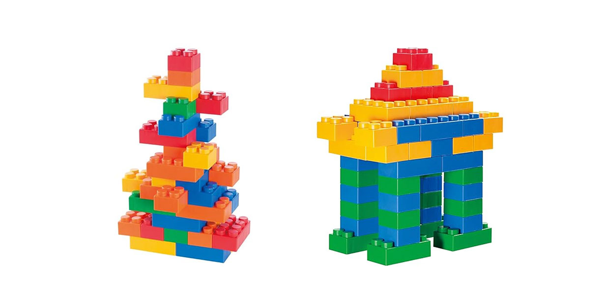
Figure 1: Two different structures built from the same basic Lego squares and rectangles

In a database, running a query means running a query plan, a tree of different operators that process and stream data. Each operator is like a Lego brick: depending on how they are connected, they compute the same result but with different performances. Much of query optimization involves swapping or moving existing operators around to form a better query plan, but on some rare occasions, a new special case operator is needed to do the job better.

Let’s walk through an example of optimizing a query by creating a specialized operator and recombining existing operators to form a query plan with superior performance.

Querying the most recent value(s)

As a time series database, one common use case is managing signal data from many devices. A common question is: “What is the signal last sent by a specified device (e.g., device number 10)?” The answer to this question (or variations of it) is often used to drive a UI or monitoring dashboard. Using SQL, a query that can answer this question is:

SELECT   …
FROM     signal
WHERE    device = 10
       AND time BETWEEN now() AND now() - interval ‘X days’
ORDER BY time DESC
LIMIT    1;

The filter time BETWEEN now() AND now() - interval ‘X days’ narrows down the question a bit: “What is the signal last sent by device number 10 for the last X days?”

While this query is simple, actual queries can be more complicated. For example, “find the average value over the last five values,” so our solution must be able to handle these more general queries as well.

It is also important that these queries return results in milliseconds, because every device owner requests values frequently. One challenge is the owner does not know when the last signal happened—it could be five minutes ago or several months ago. Thus, the value of time range X can be very large and the query runtime long. Unless users take great care writing their query, it will read and process substantial data, increasing the query return time.

Unlike traditional relational or time series databases, InfluxDB 3.0 stores data in Parquet files rather than custom file formats and specialized indexes. Our mission was to make this class of queries run in milliseconds regardless of how large the time range X is without introducing special indexes.

Runtimes before and after improvements

Before explaining our approach, let us look at the results in Figure 2. Blue represents the normalized runtimes of the queries in different time ranges before the improvements, and green represents the ones after. Queries timeout after running for 30 units, so the actual runtimes of queries that reached 30 units were even higher. As the chart shows, our improvements made large-time-range queries run hundreds of times faster and brought the runtimes of all queries down to the level requested by our customers.

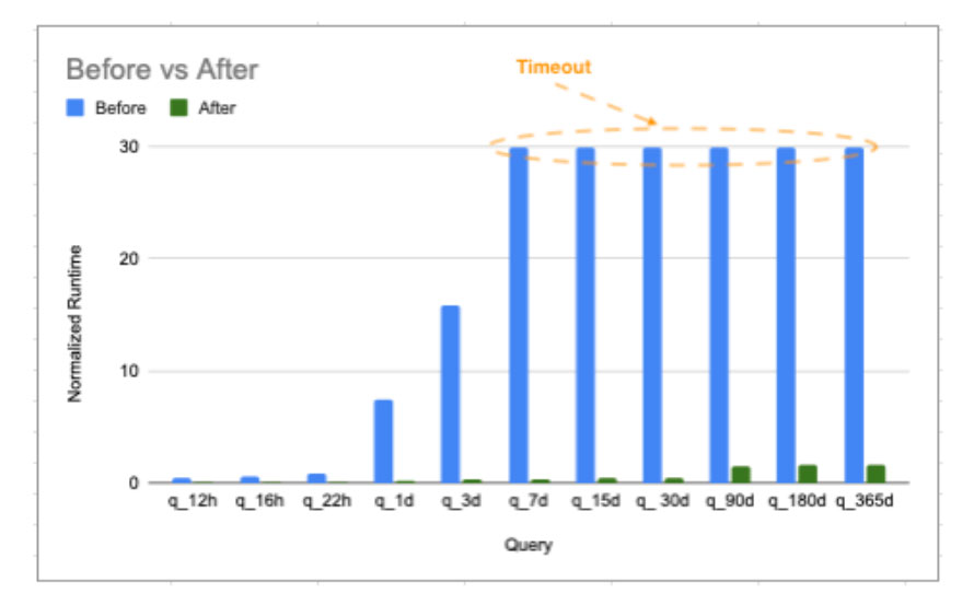
Figure 2: Query runtimes of before and after Improvements

Let’s move on to how we achieved this.

Query plan before improvements

Figure 3 shows a simplified version of the query plan before the improvements using a sort merge algorithm. We read a query plan from the bottom up. The input includes four files that four corresponding scan operators read in parallel. Each scan output goes through a corresponding sort operator that orders the data by descending timestamp. Four sorted output streams are sent to a merge operator that combines them into a single sorted stream and stops after the number of limit rows, which is 1 in this example. There are many more files in the signal table, but InfluxDB first prunes unnecessary files based on the filters of the query.

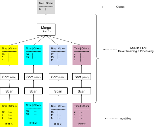
Figure 3: Query plan using sort merge algorithm

When files overlap, InfluxDB may need to‌ deduplicate data. Figure 4 shows a more accurate plan that sorts data of overlapped files, File 2 and File 3, together and deduplicates them before sending data to the sort and merge operators.

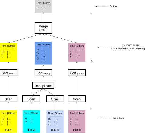
Figure 4: InfluxDB query plan using sort merge algorithm but grouping overlapped files first

The optimization described in the next section only depends on the operators at the top of the plan, and thus, the simplified plan in Figure 5 more clearly illustrates the solution. Note that we omitted many other details of the plan—for example, the Sort operator does not sort the entire file but simply retains the Top “K” rows due to the LIMIT 1 in the query.

Note that the data streams going into the merge operator do not overlap.

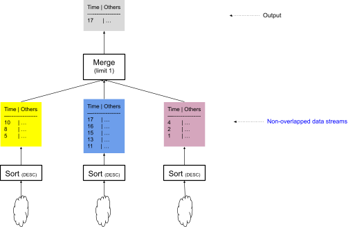
Figure 5: The top part of the plan that includes non-overlapped data streams to merge operator

Analyzing the plan and identifying improvements

Normally when merging multiple streams, all inputs must be known before producing any output (as the first row might come from any of the inputs). This implies in the above plan that we must read and sort all the input streams. However, if we know the time ranges of the streams do not overlap, we can simply read and sort the streams one by one, stopping once we find the required number of rows. Not only is this less work than‌ merging the data, but if the number of required rows is small, it is likely only a single stream must be read.

Thankfully, InfluxDB has statistics about the time ranges of the data in each file before reading them and groups overlapped files to produce non-overlapped streams, as shown in Figure 5. So, we can apply this observation to make a faster query plan without additional indexes or statistics. However, the behavior of reading streams one by one, stopping when the limit is hit is no longer a merge. We needed a new operator.

New query plan

With the observations above in mind, Figure 6 illustrates the new query plan:

1. The non-overlapped data streams are sorted by time, descending.
2. A new operator, ProgressiveEval, replaces the merge operator.

The new ProgressiveEval operator pulls data from its input streams sequentially and stops when it reaches the requested limit. The big difference between ProgressiveEval and merge operators is that the merge operator can only start merging data after all its input sort operators complete, while ProgressiveEval can start pulling data immediately after thefirst sort operator finishes.

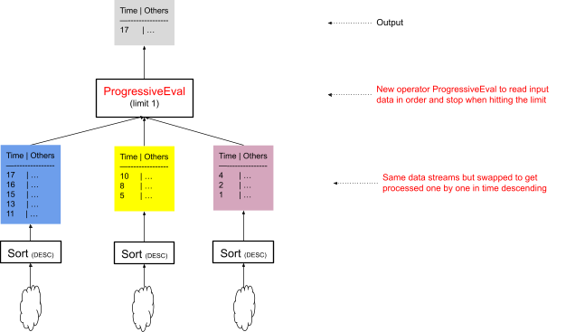
Figure 6: Optimized Query plan reads data progressively, stopping early when the limit is reached

When the query plan in Figure 6 executes, it only runs the operators shown in Figure 7. InfluxDB has a pull-based executor (based on Apache Arrow DataFusion’s Execution), which means that when ProgressiveEval starts, it will ask the first sort, which in turn asks its inputs for data. The sort then performs the sort and sends the sorted results up to ProgressiveEval.

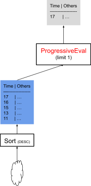
Figure 7: The needed execution operators if the latest signal of the specified device is in the latest-time-range file

Due to the device = 10 parameter, the query filters data while scanning, and we do not know in which file contains the latest signal of device number 10. In addition, because it takes time for each sort operator to complete, when ProgressiveEval pulls data from a stream, it also starts executing the next stream to prefetch data that is necessary if the first stream doesn’t contain the desired rows.

Figure 8 shows that when pulling data from Stream 1 of the first Sort, the second Sort executes simultaneously so that data from Stream 2 is ready if Stream1 does not include the requested data from device number 10. If the data from device number 10 is in Stream 1, ProgressiveEval stops as soon as it hits the limit and cancels Stream 2. If data from ProgressiveEval pulls data from Stream 2, it also begins pre-executing the Sort of Stream 3, and so on.

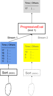
Figure 8: The actual execution operators if the latest signal of the specified device is in the latest-time-range file

Analyzing the benefits of the improvements

Let’s compare the original plan in Figure 5 and the optimized plan in Figure 8:

1. Returns Results Faster: The original plan must scan and sort all files that may contain data, regardless of the number of rows needed, before producing results. Thus, the longer the time range, the more files there are to read, and the slower the original plan is. This explains why our results show improvements for longer time ranges.
2. Fewer Resources and Improved Concurrency: In addition to producing data more quickly, the optimized plan requires far less memory and CPU—it typically will scan and sort only two files (the most recent one and pre-fetching the next most recent one). This means more queries can run concurrently with the same resources.

Type of queries that benefit from this work

At this time (March 2024), this optimization only works on one type of query, “What are the most/least recent values …?” In other words, the SQL of the query must include ORDER BY time DESC/ASC LIMIT n where ‘n’ can be any number and the time can be ordered ascending or descending. All other supported SQL queries will work but may not benefit from this optimization. We continue to work on improving them.

Conclusion

The optimization not only makes the most recent value queries faster but also reduces ‌resource usage and increases the concurrency level of the system. In general, if a query plan includes sort merge on potentially non-overlapped data streams, this optimization is applicable. We have found many query plans in this category and are working on improving them.

We would like to thank Paul Dix for suggesting this design based on the progressive scan behavior of Elastic in the ELK stack.