Monitoring Jenkins with InfluxDB

By Anais Dotis-Georgiou / Product, Use Cases, Developer
Sep 18, 2019

A critical part of DevOps is Continuous Integration/Continuous Deployment. Jenkins is the most popular Continuous Integration tool. Jenkins is an open source, Java-based automation tool that enables organizations to continuously build, test, and deploy software. Jenkins plugins (of which there are over 14,000) facilitate the automation of various development tasks. Monitoring Jenkins is critical for managing Jenkins nodes and executing your automation vision.

InfluxData’s Telegraf Jenkins Plugin gives you the following insights about your Jenkins nodes and jobs out of the box:

• Jenkins_node
  • disk_available
  • temp_available
  • memory_available
  • memory_total
  • swap_available
  • swap_total
  • response_time
• Jenkins_job
  • duration
  • result_code (0 = SUCCESS, 1 = FAILURE, 2 = NOT_BUILD, 3 = UNSTABLE, 4 = ABORTED)

InfluxDB’s free cloud tier and OSS version make InfluxDB attractive to anyone wanting to monitor Jenkins, but Flux helps to set it apart. Flux is a lightweight scripting language for querying databases and working with data. Several monitoring tools, including InfluxDB, enable you to set alerts for important build failures or correlate builds with performance metrics to resolve problems. However, Flux facilitates sophisticated analysis of Jenkins events to anticipate problems before they occur.

In this tutorial, we will learn how to use the Jenkins Plugin with InfluxDB Cloud 2.0 and OSS InfluxDB 2.0. Next, we’ll discover how easy it is to use the UI to identify any job failures. Finally, we’ll write a Flux script to isolate jobs with durations greater than two standard deviations from the mean duration of similar jobs.

Setting up the Jenkins Telegraf Plugin with InfluxDB Cloud 2.0

First, sign up for a free InfluxDB Cloud 2.0 account. After logging in, generate a Telegraf configuration for fetching Jenkins metrics:

telegraf --config jenkins_cloud.conf --input-filter jenkins --output-filter influxdb_v2.0

Now, put the appropriate config variables in the output section of the config:

[[outputs.influxdb_v2]]
 ## The URLs of the InfluxDB cluster nodes.
 ##
 ## Multiple URLs can be specified for a single cluster, only ONE of the
 ## urls will be written to each interval.
 urls = ["https://us-west-2-1.aws.cloud2.influxdata.com"]

 ## Token for authentication.
 token = "$token"

 ## Organization is the name of the organization you wish to write to; must exist.
 organization = "[email protected]"

 ## Destination bucket to write into.
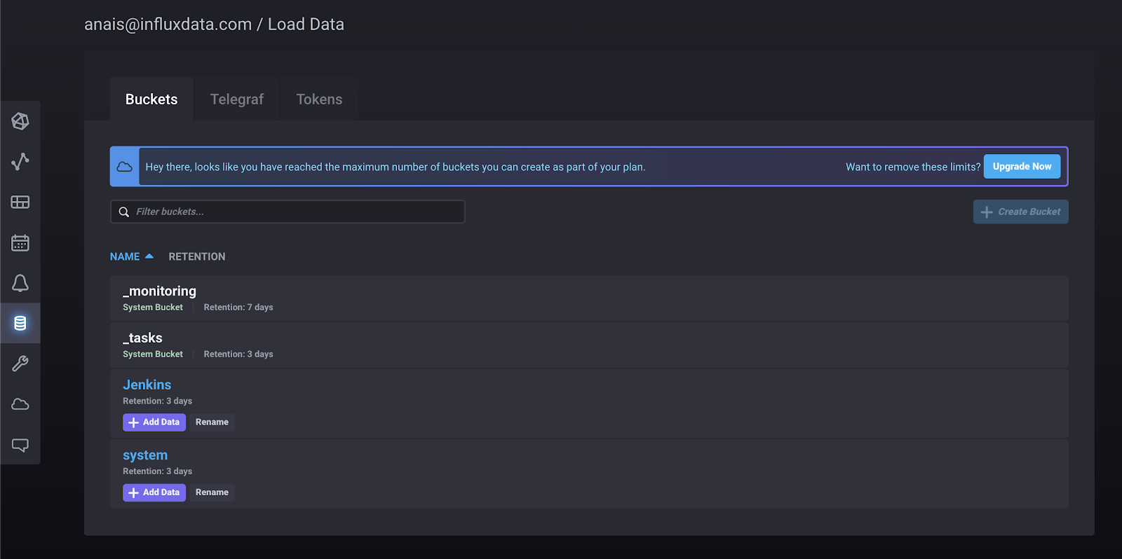
 bucket = "Jenkins"

You can create buckets, find tokens, and set the permissions in the Load Data tab at https://us-west-2-1.aws.cloud2.influxdata.com.

Next, fill out the input section of the config:

[[inputs.jenkins]]
 ## The Jenkins URL
 url = "http://localhost:8080"
 username = "admin"
 password = "$jenkins"

Finally, run Telegraf with the appropriate config:

telegraf -config jenkins_cloud.conf

Please refer to the 2.0 documentation, for more detailed instructions about setup and using the UI.

Finding failures at a glance

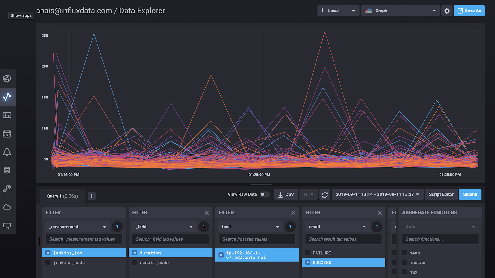
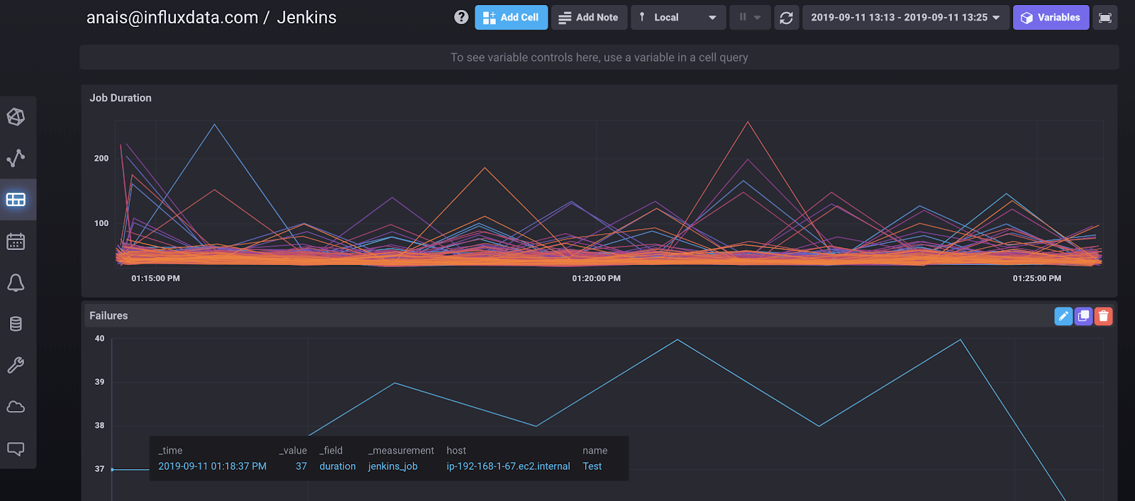
Visualizing Jenkins jobs and nodes is extremely easy with InfluxDB 2.0. I can go to the data exploration tab, and within 4 clicks, I’m able to visualize the duration of all 200 successful jobs:

I can also visualize any failures instantly:

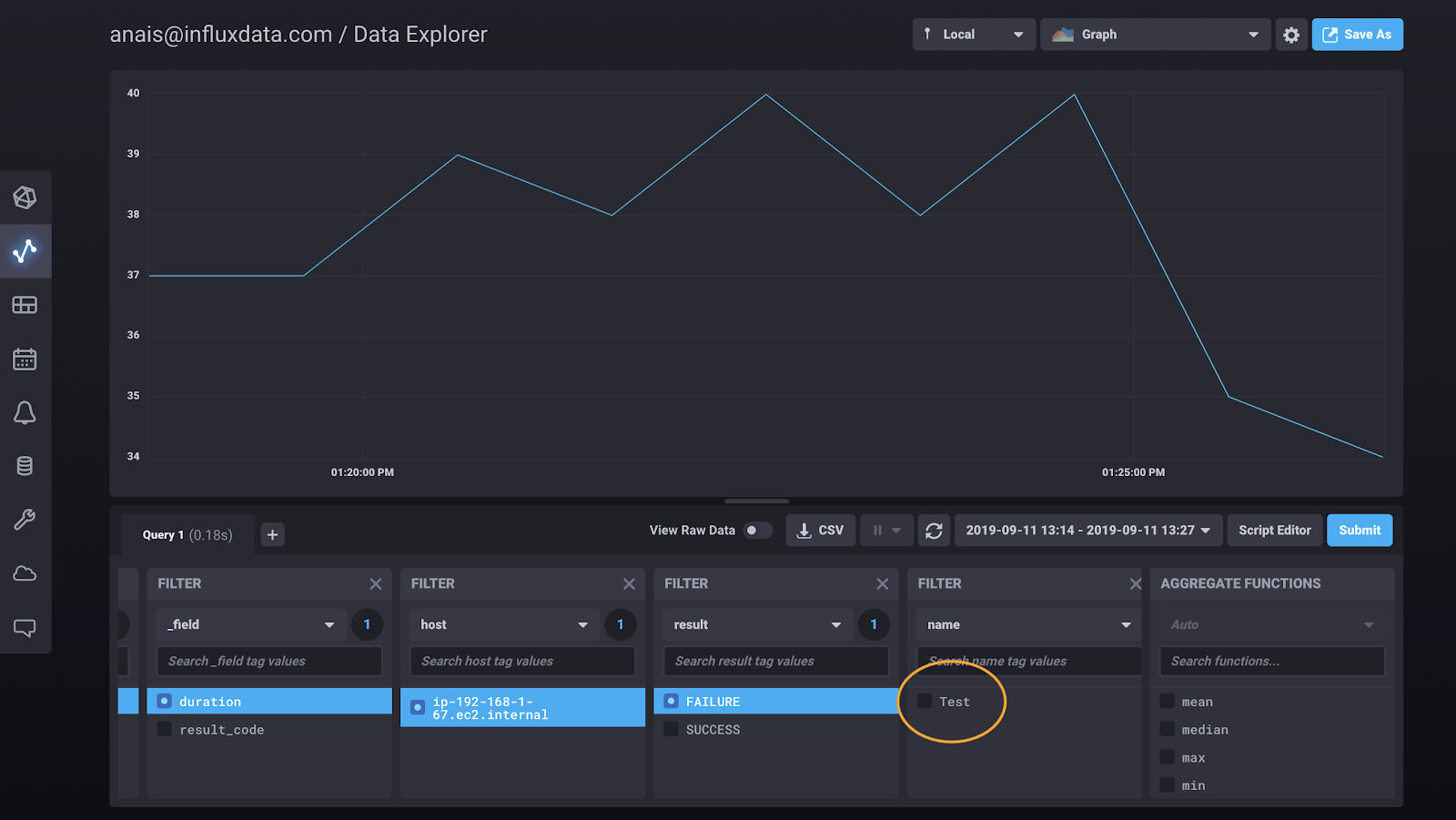
After filtering the jobs by the result code “FAILURE”, I see that my job titled “Test” failed. I can dive deeper, and isolate Job’s status to identify the time of failure.

I can also create custom dashboards with all of this information in the dashboard tab, so I can view any queries at a glance.

Identifying potentially problematic jobs with a Flux script

Being able to view job durations and job statuses is useful, but we can do more with Flux. I will take my analysis one leap further. I’ll find jobs with durations greater than two standard deviations from the mean job duration time. Then I can group those jobs by node to identify potentially problematic nodes.

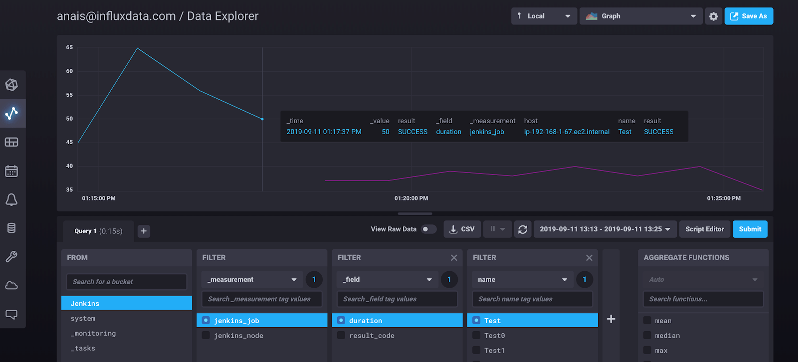
First, let’s take a look at our data. The following query lets me view the build duration of all of my jobs.

duration = 
  from(bucket: "Jenkins")
  |> range(start: v.timeRangeStart, stop: v.timeRangeStop)
  |> filter(fn: (r) => r._measurement == "jenkins_job")
  |> filter(fn: (r) => r._field == "duration")
  |> toFloat()
  |> keep(columns: ["_value", "name", "_time"])
  |> set(key: "mykey", value: "myvalue")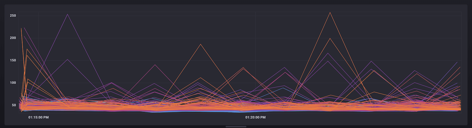

<figcaption> Graph view of the “duration” stream</figcaption>

<img class=”wp-image-237015 size-full” src=”https://w2.influxdata.com/wp-content/uploads/jenkins-table-view-of-duration-stream.png” alt=”Jenkins - table view of the “duration” stream” width=”1600” height=”385” /><figcaption> Table view of the “duration” stream</figcaption>

From visual inspection, we notice that most of the jobs have an average build duration time of approximately 50ms. However there are quite a few jobs that took much longer to build. The goal of this exercise will be to isolate those jobs. The toFloat() function is used to help apply a map() function later. The keep() function eliminates unwanted columns and  cleans up the table stream. The set() function is applied to enable a join later.

First, the mean is calculated with:

mean = 
  from(bucket: "Jenkins")
  |> range(start: v.timeRangeStart, stop: v.timeRangeStop)
  |> filter(fn: (r) => r._measurement == "jenkins_job")
  |> filter(fn: (r) => r._field == "duration")
  |> group()
  |> mean(column: "_value")
  |> keep(columns: ["_value", "name", "_time"])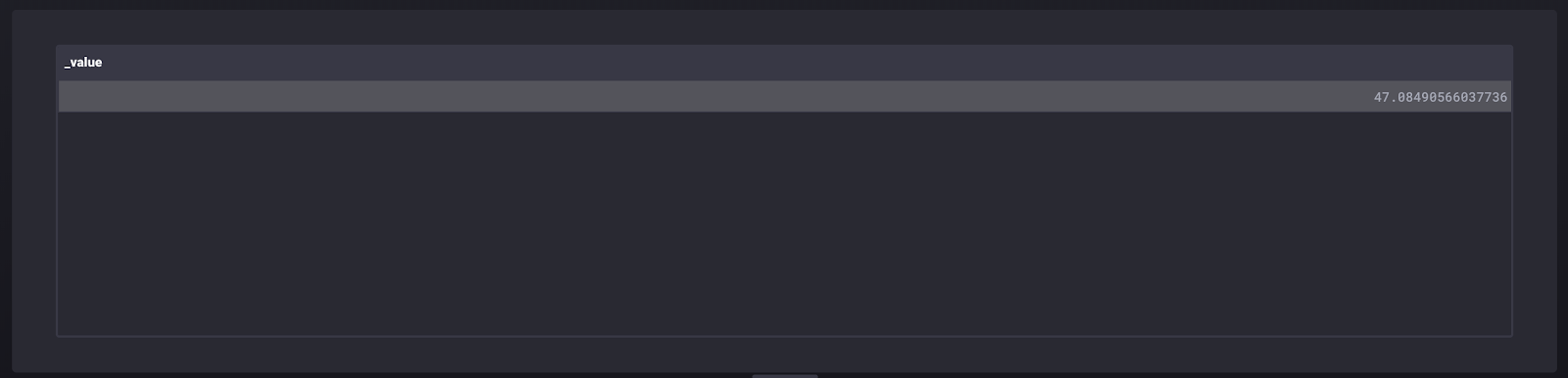

<figcaption> Table view of the “mean” stream</figcaption>

We see that the mean is close to 50, as expected.

Next, the standard deviation is calculated with:

duration_stddev = 
  from(bucket: "Jenkins")
  |> range(start: v.timeRangeStart, stop: v.timeRangeStop)
  |> filter(fn: (r) => r._measurement == "jenkins_job")
  |> group()
  |> stddev(column: "_value", mode: "sample")
  |> keep(columns: ["_value", "name", "_time"])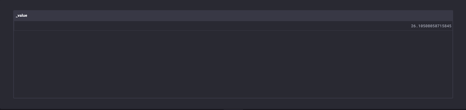

<figcaption> Table view of the “duration_stddev” stream</figcaption>

Next we will calculate a “ _limit”, our anomaly threshold, as two standard deviations away from the mean. This calculation is achieved by joining together our standard deviation and mean tables and then computing the limit.

normal = 
  join(tables: {duration_stddev: duration_stddev , mean: mean}, on: ["name"])
  |> map(fn: (r) => ({r with _limit:(r._value_duration_stddev*2.0 + r._value_mean)}))
  |> keep(columns: ["_limit", "mykey"])
  |> set(key: "mykey", value: "myvalue")

<img class=”size-full wp-image-237022” src=”https://w2.influxdata.com/wp-content/uploads/Table-view-of-the-normal-stream.png” alt=”Table view of the “normal” stream” width=”1600” height=”385” /><figcaption> Table view of the “normal” stream</figcaption>

We can see how the set() function adds an extra column to the table stream, as was applied to the “duration” stream .

Now we can find our anomalous jobs. We join together the “duration”  and “normal” streams and define the anomaly as being any value greater than the limit.

anomaly = 
  join(tables: {duration: duration , normal: normal}, on: ["mykey"])
  |> map(fn: (r) => ({r with _anomaly:(r._value - r._limit)}))
  |> filter(fn: (r) => r._anomaly > 0)
  |> keep(columns: ["_anomaly", "name", "_time"])

<img class=”size-full wp-image-237023” src=”https://w2.influxdata.com/wp-content/uploads/scatter-plot-view-of-the-anomaly-stream.png” alt=”Scatter Plot view of the “anomaly” stream” width=”1600” height=”758” /><figcaption> Scatter Plot view of the “anomaly” stream</figcaption>

We can see that around 20 jobs have build times that exceeded our limit. The symbol shape and symbol color have been configured to be grouped by job name, so we can easily identify troublesome jobs.

Considerations

Please note that the data used in this tutorial is dummy data generated to demonstrate some Flux capabilities. This helps explain why such a seemingly high number of jobs had “anomalous” build times. I created a very simple Job with the Jenkins UI and copied that job 200 times using the Python-Jenkins CL. The Python script and Telegraf config is in this repo.

Throughput and conclusion

The InfluxDB UI enables even those of us who don’t code to quickly build Flux scripts and visualize Jenkins metrics. Flux also allows us to perform sophisticated analysis on Jenkins metrics in order to identify potentially problematic nodes and isolate job failures easily. The InfluxDB Cloud 2.0 free tier allows you to do so with really good throughput. Considering the restrictions and assuming you configure Telegraf to node_exclude = [ "*" ],  you can still write over 25000 points containing job metrics every 5 minutes, or 800 per second. I hope you enjoyed this tutorial. If you run into hurdles please share them on our community site or Slack channel.