OpenTelemetry Tutorial: Collect Traces, Logs & Metrics with InfluxDB 3.0, Jaeger & Grafana

By Jay Clifford / Jacob Marble / Use Cases, Product
May 05, 2023

Here at InfluxData, we recently announced InfluxDB 3.0, which expands the number of use cases that are feasible with InfluxDB. One of the primary benefits of the new storage engine that powers InfluxDB 3.0 is its ability to store traces, metrics, events, and logs in a single database.

Each of these types of time series data has unique workloads, which leaves some unanswered questions. For example:

• What schema should I follow?
• How do I convert my traces to line protocol?
• How does InfluxDB connect with the larger observability ecosystem?

Luckily this is where our work within OpenTelemetry comes into play. If you want to learn more about what OpenTelemetry is, we recommend this blog by Charles Mahler. However, the aim of this blog is to take you through a working example of OpenTelemetry and InfluxDB 3.0.

Running the demo

Let’s start with the fun part by running the demo and then discussing the theory behind it. Here is the demo we are going to deploy:

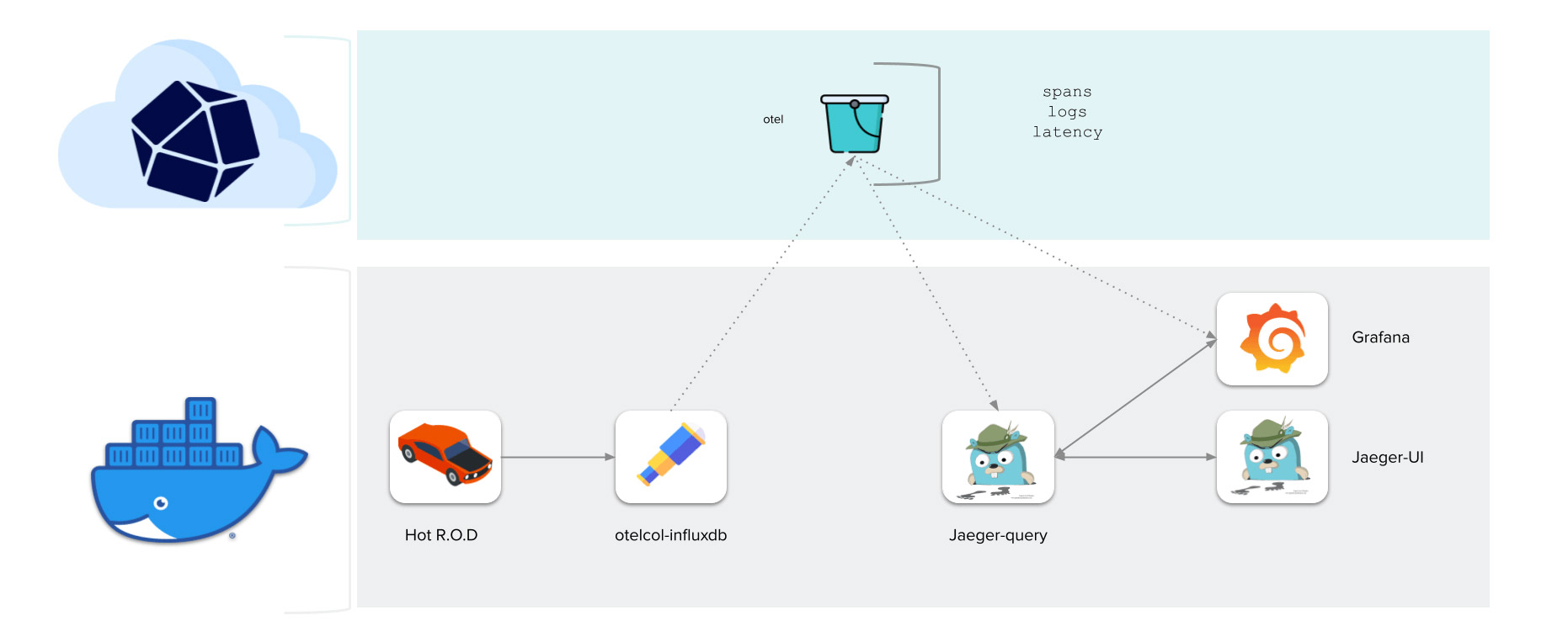
This demo uses Hot R.O.D. to simulate traces, logs, and metrics. We then use OpenTelemetry Collector to collect that data and write it to InfluxDB 3.0. Finally, we use Grafana and Jaeger UI to visualize this data in a highly summarized view.

To run the demo you can use this KillerCoda demo environment.

Simply create an account and follow the tutorial to run through the demo without worrying about a local installation. For local installs, we have all the info you need in a GitHub repo, so check out the repository readme for up-to-date installation instructions.

Walkthrough

Let’s run through the demo with Killercoda so you can see what to expect:

1. You will see the demo provisioning script ticking away on the first load. It shouldn’t take too long. You will know it finished loading once InfluxDB OTEL Demo appears.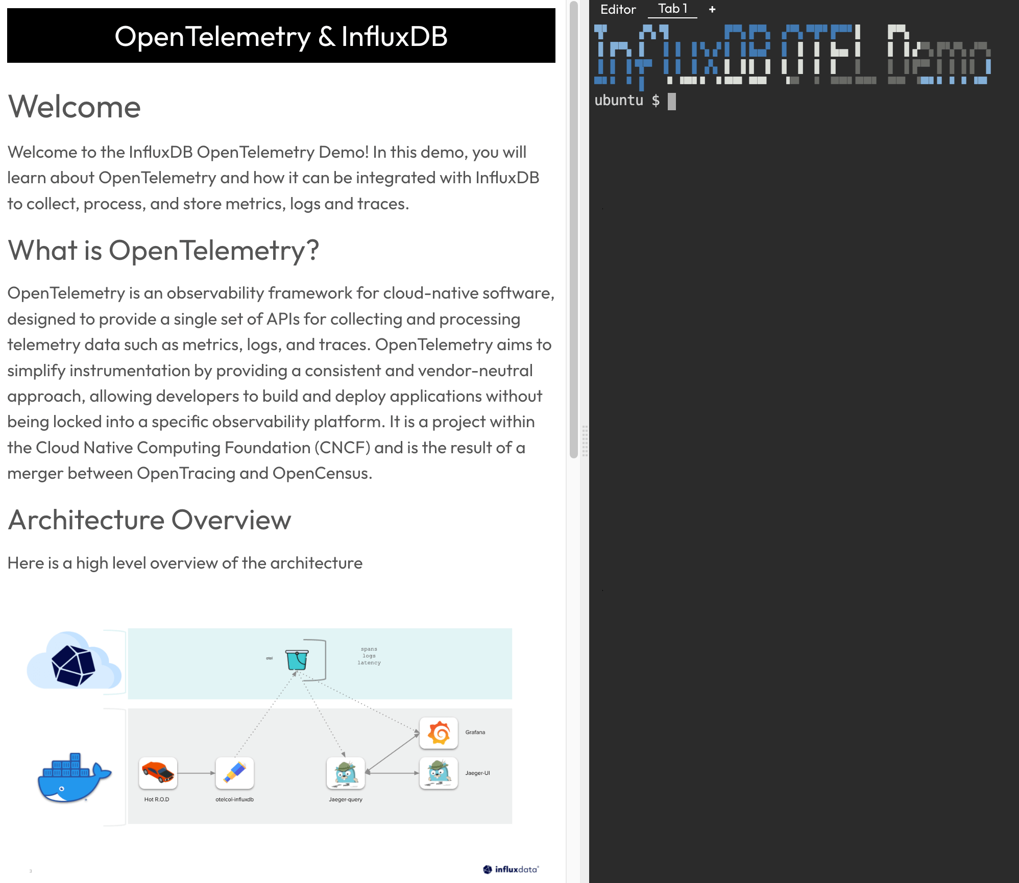
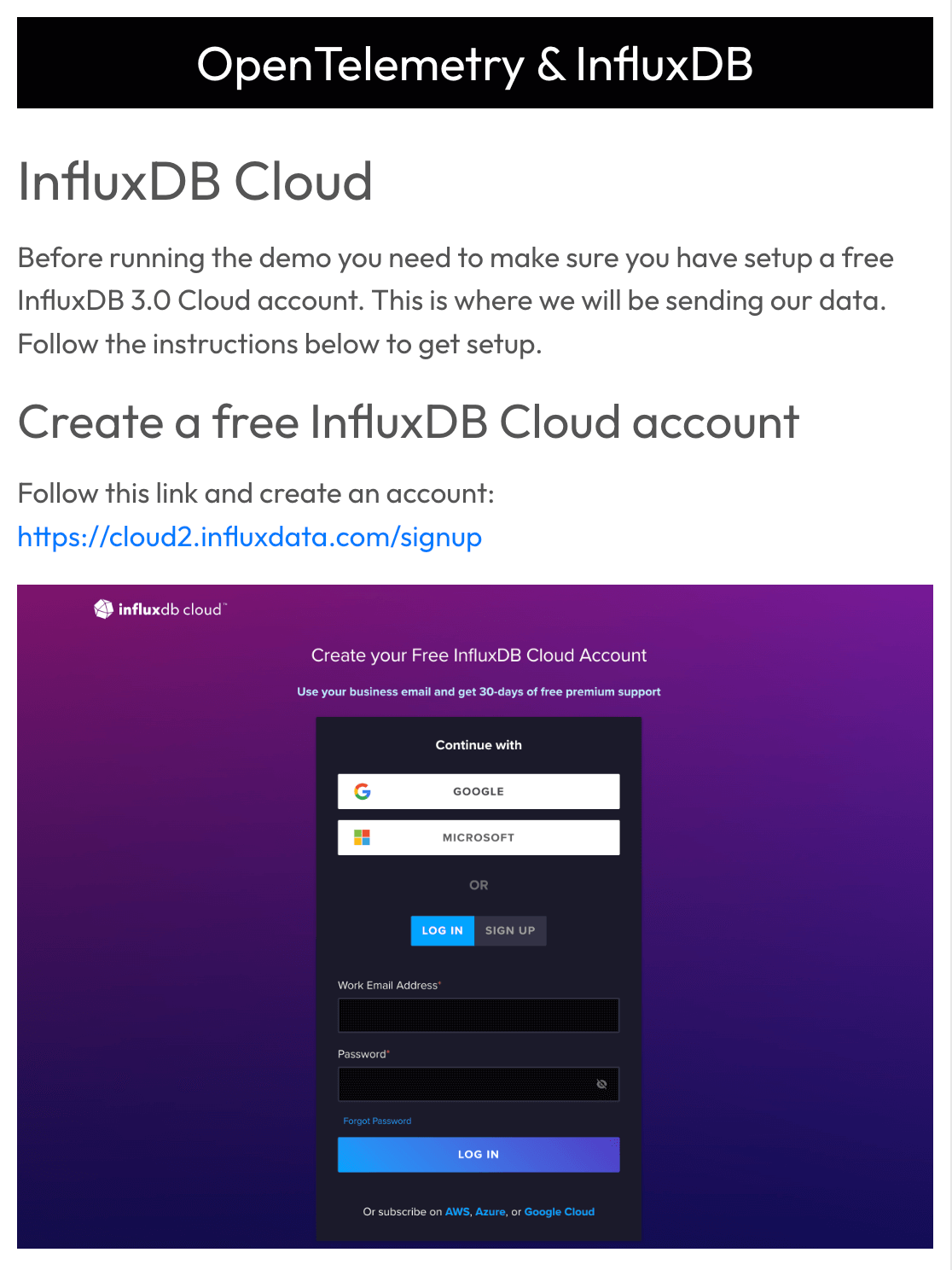
2. If you don’t already have one, follow the steps to create a free InfluxDB 3.0 Cloud account for the demo. Make sure to follow the instructions for creating a bucket in InfluxDB called otel and generating a read-and-write token for the new otel bucket.
3. Next, we provide credentials for InfluxDB 3.0 so the demo can write and query from our otel bucket. To do this, select the Editor tab within Killercoda and navigate to influxdb-observability/.env. This is where we update our connection credentials. Note: Make sure to update INFLUXDB_ADDR to point to your InfluxDB Cloud region. Also, remove any protocols from the address (e.g., HTTPS://).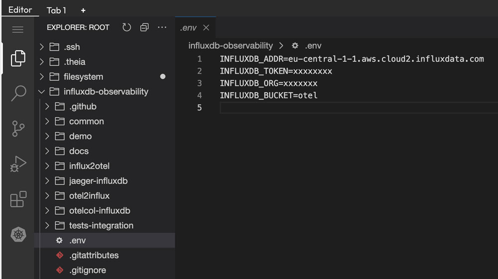
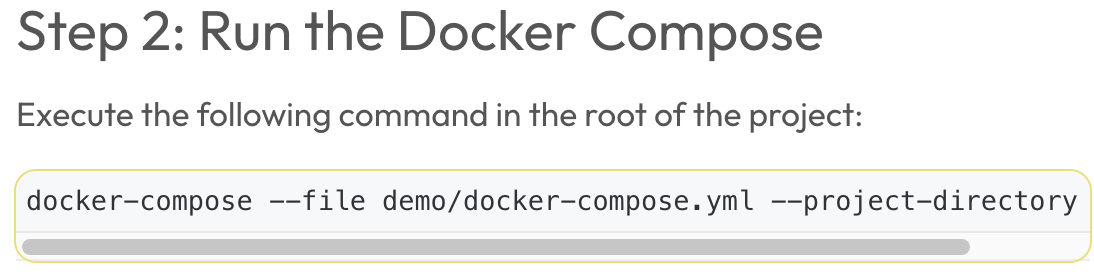
4. Once we finish updating the environment, we can start the demo. Simply click this command to spin up the demo: docker-compose --file demo/docker-compose.yml --project-directory
5. Now we get to the fun part! Let's generate some traces. First of all, let's open the HotROD application. Within a local installation, this runs via localhost:8080. To access this address in Killercoda, follow the hyperlinks provided in the screenshot below.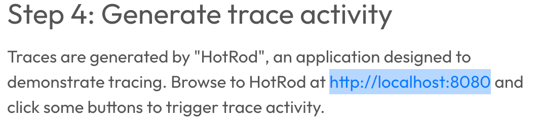
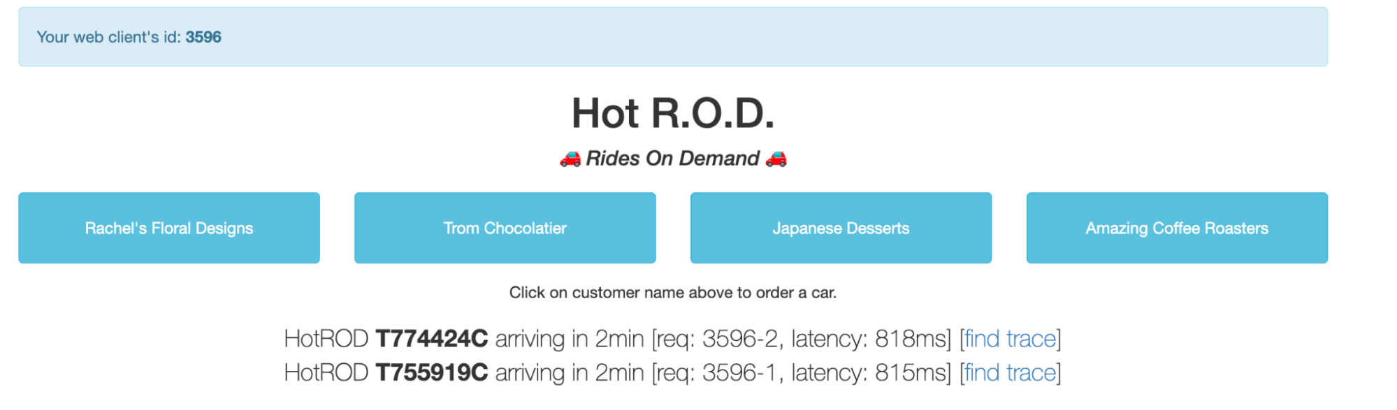
6. From there we can start generating traces by clicking on the different buttons. Each one simulates ordering a car for the indicated task, which triggers the background service calls and creates the trace.
7. If you head over to your InfluxDB 3.0 Cloud instance, you can explore the otel bucket schema to see how we translate the OpenTelemtry data structure into InfluxDB’s line protocol, which consists of measurements, tags, and fields. (Note: We will cover line protocol more in-depth in the next blog.)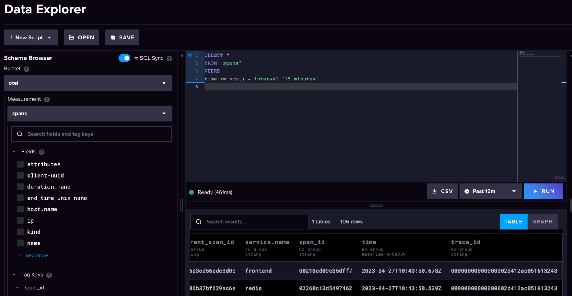
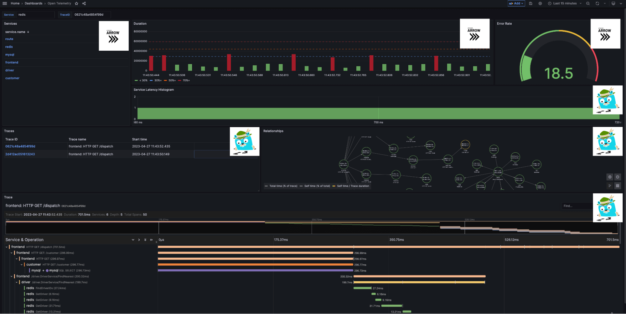
8. If we head back to our Killercoda instance and open up Grafana, we can explore our OpenTelemetry dashboard and configuration.

Grafana explained

This section breaks down some of the key features of the Grafana dashboard. Let’s start with the data sources.

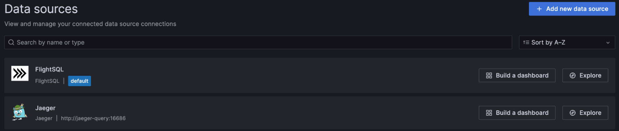
As you can see, we connected to two data sources – Flight SQL and Jaeger. Both sources pull data directly from InfluxDB 3.0, but we will discuss how they work and their differences in more detail in the next blog. For now, you just need to know the following:

• Flight SQL – This is the direct SQL query interface for InfluxDB 3.0. It is great for general-purpose time series-based queries and metrics summaries.
• Jaeger – This functions as the bridging interface for metrics, logs, and traces between InfluxDB 3.0 and Grafana visualizations.

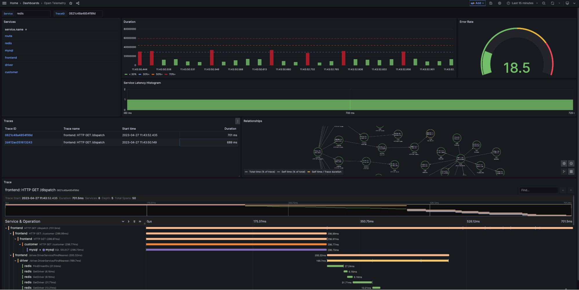
Let’s look at our dashboard again and map our data sources to the different panels.

We use Flight SQL to generate our general-purpose navigation and summary overviews:

• Services queries InfluxDB for all unique services found within the otel bucket. We use the service names as data links for the rest of our visualization. For example, clicking redis filters my summary results and trace list to only include the service redis.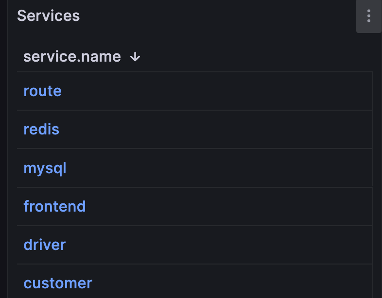
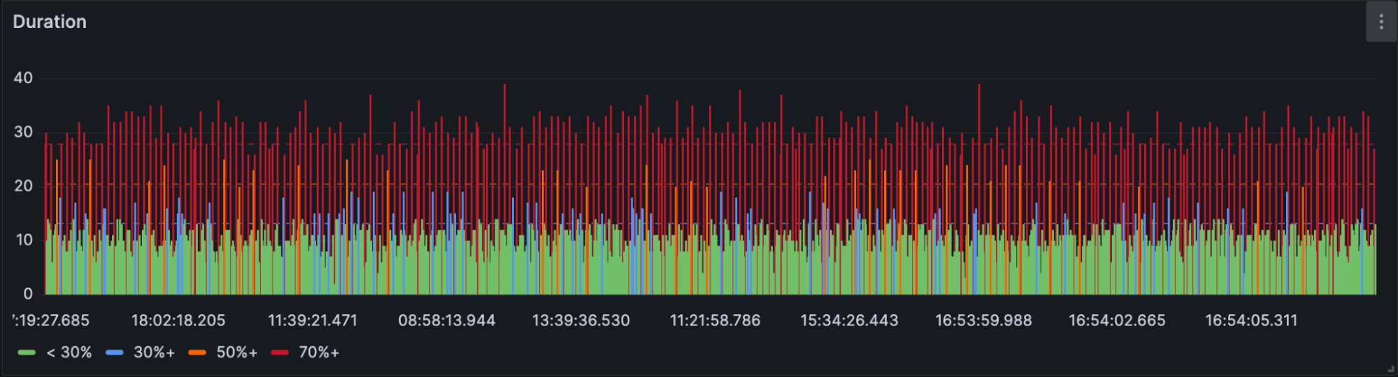
• Duration returns the duration in nanoseconds of each spanID over the selected time period. As part of our SQL query, we convert this value to seconds to improve readability.
• Error Rate calculates the service error rate, as a percentage, based on the number of errors flagged in the otel.status column.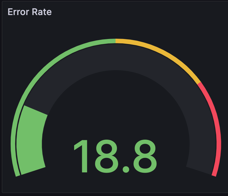

We use Jaeger to drill into our traces with the following visualizations:

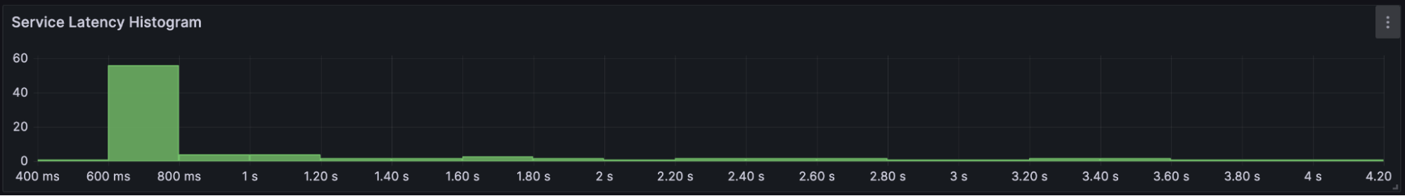
• Service Latency Histogram creates a histogram based on the latency of traces within the service. This panel groups trace spans based on their detected latency range.
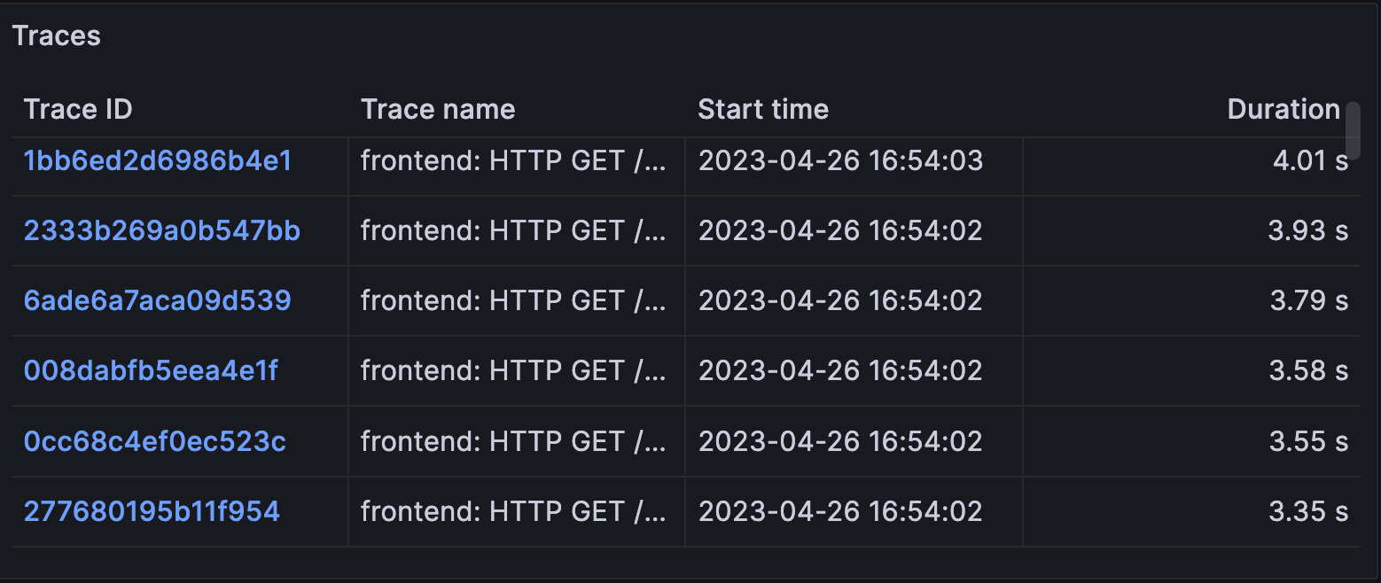
• Traces provides a table of traces associated with the selected service. The table includes trace name, start time, and duration. Users can select TraceID’s to generate the next two visualizations: Relationships and Trace.
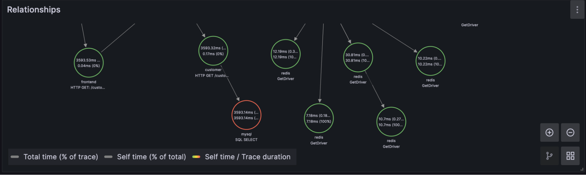
• Relationships: After selecting a TraceID in the Traces panel, users can navigate span relationships within the trace using the span tree. We’ll have more on this in the next blog.
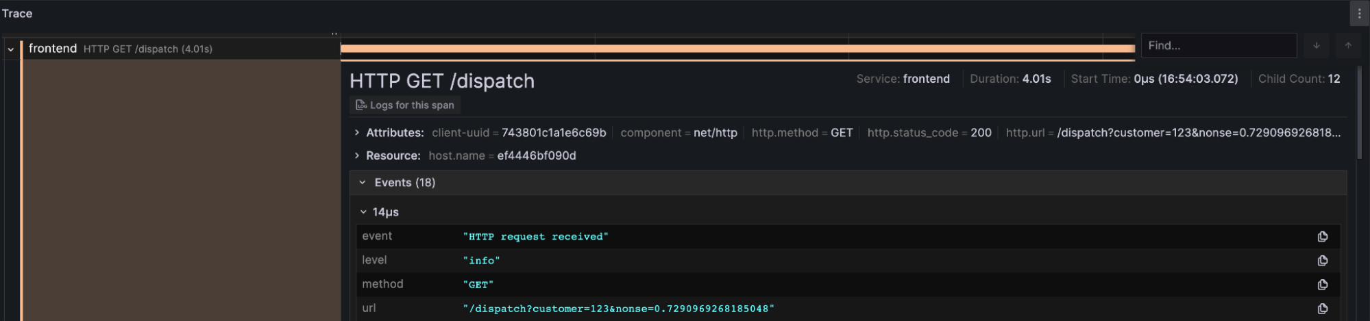
• Trace: This panel allows users to navigate raw trace data for the selected TraceID and its associated log data.

Conclusion

We hope this tutorial provides you with a solid foundation to learn more about OpenTelemetry and how InfluxDB 3.0 will play a pivotal role in future observability solutions. Stick around for the next blog where we will delve into the theory of OpenTelemtry, breaking down each component in the demo architecture and discussing data schemas. Until then play with the demo, fork the repo, and see if you can apply these components to your own use case. If you have any questions please do not hesitate to reach out to us on Slack.