Pandas Profiling: A Detailed Explanation

By Community / Developer
Jan 08, 2024

If you’ve dipped your toes into programming, chances are you’ve encountered Python. A friendly and versatile language, Python is used for manipulating data and machine learning with various libraries and modules so that developers and data scientists can carry out multiple tasks.

When it comes to data analysis, you first need to explore your data by carrying out exploratory data analysis (EDA). EDA can be hectic, and it can feel like you’re navigating a maze blindfolded, so Python offers a pandas profiling package to streamline it. In this article, we’ll cover pandas profiling, or ydata-profiling as it’s called now, and how to use it.

What Is Pandas Profiling?

Pandas profiling is an open-source Python package or library that gives data scientists a quick and easy way to generate descriptive and comprehensive HTML profile reports about their datasets. The most exciting thing is that it generates this report with just a single line of code.

The information it provides includes missing values, duplicate records, categorical and numeric records, correlations, and histograms. This information makes it easy to understand the data and identify potential issues. We’ll explore some examples later in this post.

How Does Pandas Profiling Work?

Pandas profiling is available on the Python Package Index (PyPI) and generates profile reports from a Pandas DataFrame in either HTML or JSON format.

It is, however, essential to know that pandas profiling is now known as ydata-profiling. This package is also built on pandas and NumPy. Regarding data structure, ydata-profiling supports tabular data, time series text, and image data.

Just like every other Python package, you can easily install ydata-profiling can be easily installed via the pip package manager using the command below:

pip install -U ydata-profiling

You can also install it via the Conda package manager. You can find more information on the Conda docs.

conda install -c conda-forge ydata-profiling

Installing it locally on Google Colab or Kaggle is also an option. You will, however, need to restart the kernel or runtime for the package to work.

import sys

!{sys.executable} -m pip install -U ydata-profiling[notebook]

!jupyter nbextension enable --py widgetsnbextension

How to Import and Generate a Report with ydata-profiling

To generate a report with ydata-profiling, run the command below:

#importing ydata-profiling

From ydata_profiling import ProfileReport

#generating a report

ProfileReport(df, kwargs)

In this syntax:

df represents your Pandas DataFrame, which is a two-dimensional tabular data set; kwargs represent all the optional keyword arguments Pandas profiling offers users for customization.

A few of these optional arguments include the following:

• Samples allow you to use just a subset for profiling. This is useful for large datasets.

sample = df.sample(1000)

ProfileReport(sample, minimal=True)

• Minimal allows a minimalistic report. You just have to set it as True.

ProfileReport(sample, minimal=True)

• Title allows you to give your profiling report a title.

ProfileReport(df, title="My Report")

• Correlations allows you to set the correlation metrics and thresholds for the profiling report.

ProfileReport(df, title="My Report", correlations=None)

Using the ydata-profiling Pandas Profiling Package

Now that you’ve installed the package, let’s look at how you can use it with examples.

This tutorial will use Google Colab and the Bitcoin historical datasets from our sample GitHub repository. You can also get it from the sample data section of InfluxDB documentation.

Generating a simple report

You can generate a simple report by importing ydata-profiling and using the ProfileReport method to generate the chart.

from ydata_profiling import ProfileReport

profile = ProfileReport(data)

profile

A standard ydata-profiling report comes with five main sections.

1. Overview: has three report tabs: Overview, Warnings, and Reproduction.
   • Overview shows statistics like the number of sizes, missing cells, and duplicate rows.
   • Alerts preview any warnings like columns with unique values, cardinality, and skewness of the variables.
   • The Reproduction page shows information about the report generation, like the start and end time and the software version.
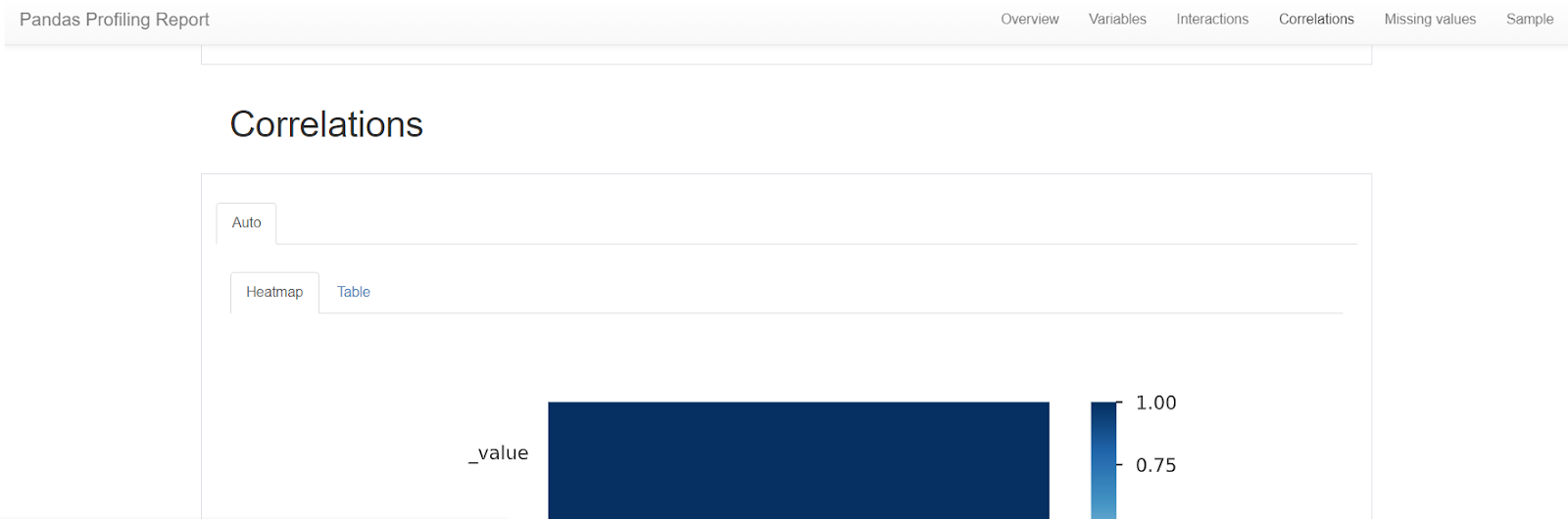
2. Variables report consists of a detailed analysis of each variable (columns). This output depends on whether the column you pick is categorical or numerical. Some of the information in this section includes distinct values, missing values, means, histograms, and the number of characters. This section also gives a more detailed overview if you click the More Detail toggle button. 3. Correlations provide correlations in the data. Ydata-profiling gives you access to five types of correlation coefficients: pearson, spearman, Kendall, phi_k, and cramers. 4. Missing Values provide visualizations for the missing values present in the data set. You get a count (bar) and matrix plot by default. 5. The Sample page displays the first and last few rows of the data set.
   

Setting a dataset description

When working with data, a description can give you an idea of what the report is about. You can set a description, copyright_holder, copyright_year, and URL for your data.
Here’s an example of how you can set a description for your data:

from ydata_profiling import ProfileReport

    profile = data.profile_report(

        title="Bitcoin Profiling Report",

        dataset={

            "description": "This profiling report was generated by Benny Ifeanyi using ydata_profiling.",

            "copyright_holder": "InfluxDB",

            "copyright_year": 2023,

            "url": "https://github.com/influxdata/influxdb2-sample-data/blob/master/bitcoin-price-data/bitcoin-historical-annotated.csv",

        },

    )

    Profile

Playing around with ydata-profiling optional keyword arguments

Now we’ll show you how to create a simple report and how you can use the keyword arguments.  First, as seen below, the title argument can be used to add a title.

from ydata_profiling import ProfileReport

    profile = ProfileReport(data, title="Bitcoin Profiling Report")

    profile

You can use the missing_diagrams argument to visualize the missing data in your report. You can visualize it as either a bar, matrix, or heatmap. By default, these visualizations are all TRUE.

from ydata_profiling import ProfileReport

    profile = ProfileReport(data, title="Bitcoin Profiling Report", missing_diagrams={"matrix": False,})

    profile

The code above disables the matrix missing value visual.

Profiling time series data set

Ydata_profiling can analyze your time series data. You can enable this by setting tsmode to True. Once you do that, ydata_profiling will identify your time data and create autocorrelation. This is helpful for finding seasonality and trends in your data.

You should also explore time series databases like InfluxDB to optimize the storing and querying of time series data.

Here’s the code to profile your time series data:

from pandas_profiling import ProfileReport

    profile = ProfileReport(data, title="Bitcoin Profiling Report", tsmode=True, sortby="_time")

    profile

In the code above, the tsmode argument was set to true to enable time series analysis, and the sortby argument was used to sort the time column.

Profiling and handling sensitive data

If confidentiality is super important, you can use the sensitive argument to only show the data in an aggregated view. This way, individual records remain private.

from ydata_profiling import ProfileReport

    profile = ProfileReport(data, title="Bitcoin Profiling Report", sensitive=True)

    profile

Profiling big data

Comprehensively summarizing and generating this report can take a while when your data sets are large. To speed up the process, ydata-profiling offers some solutions.

A good starting point is to use the minimal keyword argument. This argument turns off the most expensive computations.

from ydata_profiling import ProfileReport

    profile = ProfileReport(data, title="Bitcoin Profiling Report",  minimal=True)

    profile

Another method is the sample argument. This method allows you to select a subset of your data for analysis while ensuring that it’s representative of the entire data set.

from ydata_profiling import ProfileReport

    sample = data.sample(1000)

    profile = ProfileReport(sample, title="Bitcoin Profiling Report", minimal=True)

    profile

Similarly, you can use the frac function to pick a percentage of your data.

sample = data.sample(frac=0.05)`

    profile = ProfileReport(sample, title="Bitcoin Profiling Report", minimal=True)

    profile

However, for a much smaller data set, you can use the explorative argument for deeper profiling. This will, however, take a long time for big data.

from ydata_profiling import ProfileReport

    profile = ProfileReport(data, title="Profiling Report", explorative=True)

    profile

Saving your profiling report

Now that you’ve learned how to generate reports with a single line of code, try saving a report. This is important when you want to export the report or integrate it with another system.

You can import the report in HTML or JSON format using the .to_file() function.

from ydata_profiling import ProfileReport

    profile = ProfileReport(data, title="Bitcoin Profiling Report")

    profile.to_file("output.html") #this saves it as a HTML file

    profile.to_file("output.json") #this saves it as a JSON file

Now that you’ve seen ydata-profiling in various examples, it’s time to get your hands dirty by trying one of our sample datasets.

What Are Some Alternatives to ydata-profiling?

There are a few other alternatives to ydata-profiling.  Let’s explore some using the _time, _value and crypto column of the Bitcoin historical dataset from our sample data GitHub repository.

df.describe: This pandas method only provides basic summary statistics like the central tendency. It doesn’t provide insights into other aspects of your data, like missing values or categorical variables.

df = pd.DataFrame(data)

    summary = df.describe()

    print(summary)

sweetVis: Like ydata-profiling, this generates a comprehensive report about your data. You can do so by running the command below.

pip install sweetviz

    import sweetviz as sv

    report = sv.analyze(data)

    report.show_html('report.html')

    from IPython.display import HTML

    HTML(filename='report.html')

DataPrep:: This also creates comprehensive data reports with one line of code. You can do so by running the command below:

pip install -U dataprep

    import pandas as pd

    from dataprep.eda import create_report

    create_report(data)

You can explore this Github gist with the output and the code snippets.

What Are Some Disadvantages of ydata-profiling?

The bigger your data set, the longer ydata-profiling takes to generate your report. You can, however, tackle this with the following: * Using the samples argument to pick a subset of the data to profile. * Using the minimal argument to generate a simplified minimalistic report.

We looked at these arguments and their syntax earlier in this tutorial’s big data profiling section.

Key Takeaways

In this tutorial, you learned about pandas profiling and how it has been modified into ydata-profiling. You saw how to use this package to generate a simple report with just a line of code. Additionally, you saw how to compare data sets, use the optional key arguments, and much more. We also explored some alternatives and how to handle ydata-profiling’s disadvantages.

As mentioned, by using this package you can effectively carry out EDA with your data. This will enable you to manipulate and build Python projects with InfluxData’s Python support and API documentation.

To learn more about InfluxDB, check out our blog and university, which can provide you with the skills to build powerful applications that use real-time data.

This post was written by Ifeanyi Benedict Iheagwara. Ifeanyi is a data analyst and Power Platform developer who is passionate about technical writing, contributing to open source organizations, and building communities. Ifeanyi writes about machine learning, data science, and DevOps, and enjoys contributing to open-source projects and the global ecosystem in any capacity.