Time Series, InfluxDB, and Vector Databases
By
Anais Dotis-Georgiou
Mar 26, 2024
Developer
Navigate to:
Integrating time series data with the power of vector databases opens up a new frontier for analytics and machine learning applications. Time series data, characterized by its sequential order and timestamps, is pivotal in monitoring and forecasting across various domains, from financial markets to IoT devices. InfluxDB, a leading time series database, excels in handling such data with high efficiency and scalability.
On the other side of the spectrum lies Milvus, a highly versatile vector database designed to manage and query high-dimensional vector data, enabling advanced similarity searches crucial for AI-driven insights.
This blog post explores the seamless synergy between InfluxDB and Milvus, guiding you through the process of querying data from InfluxDB, normalizing the data, converting it into vectors, and writing it into Milvus.
Finally, we perform a similarity search on our time series to identify whether the monitored conditions are familiar. By harnessing the strengths of both databases, we unlock a comprehensive approach to managing and leveraging complex datasets for cutting-edge applications.
Requirements
In order to run this example, you’ll need the following:
- Docker
- Jupyter Notebooks
- A free-tier InfluxDB Cloud instance
You’ll need to gather the following credentials from your InfluxDB instance:
- Bucket/database
- Token
- URL
To run this example, clone the following repo and follow the instructions in the README.md. In this step, you’re building and starting the Milvus container and running the Jupyter Notebook.
What is a vector database?
Vector databases are specialized storage systems designed to efficiently handle vector data (arrays of numbers representing complex data points such as images, text, or audio features). These databases excel in storing, indexing, and querying high-dimensional vectors, typically generated by machine learning models or algorithms. The core reason for their popularity is their exceptional ability to perform similarity searches; they can quickly identify vectors most similar to a query vector, making them indispensable for applications like recommendation systems, image and speech recognition, and natural language processing.
The rise of AI and machine learning has fueled the need for efficient similarity search mechanisms, propelling vector databases into the spotlight. They use advanced indexing techniques to manage the curse of dimensionality—a challenge in high-dimensional spaces where traditional database approaches struggle with performance. This efficiency allows for real-time querying even in massive datasets, enhancing user experience and the effectiveness of machine learning models.
Moreover, vector databases facilitate a nuanced understanding and handling of data, moving beyond simple keyword searches to embrace the complexity of real-world data. This capability enables applications to deliver more accurate and relevant results, driving the growing adoption of vector databases in various industries aiming to leverage AI and machine learning innovations for competitive advantage.
A TSDB and vector database scenario
To better understand the relationship between time series databases (TSDB) and vector databases, it’s helpful to contextualize their use within an example scenario. Imagine you’re developing a platform that offers real-time traffic monitoring and pattern recognition to improve city traffic management. Specifically, you want to create a solution that identifies when traffic conditions are operating anomalously and determines the type of traffic anomaly present, like an accident, traffic, or construction. InfluxDB would store the time series data from the sensors, while Zilliz would store the image data and manage the search indices for complex queries. In this scenario, you could continuously monitor traffic data, like average speed and vehicle count, in InfluxDB. You might also be collecting traffic image data in Milvus. When traffic conditions fall outside the norm, you send this anomalous traffic data to Milvus. Then, you perform a similarity search in Milvus to identify the type of anomaly.
This post will highlight how to:
- Generate dummy traffic data
- Write it to InfluxDB v3
- Query it from InfluxDB v3
- Normalize and vectorize the data (a lot of this code for this section comes from the following tutorial)
- Insert it into Milvus
- Perform a similarity search with a new time series to try and identify whether it resembles a past time series
Beginning steps
First, we’ll start by generating some dummy time series traffic data:
def generate_sensor_data(anomaly_type, speed_limit, vehicle_count_range, avg_speed_range, rows=500):
    """
    Generate a DataFrame with sensor data including vehicle count, avg speed, anomaly type, and timestamp.

    Parameters:
    - anomaly_type: string, the type of traffic anomaly (traffic, accident, road work)
    - vehicle_count_range: tuple, the range (min, max) of vehicle count
    - avg_speed_range: tuple, the range (min, max) of average speed
    - rows: int, number of rows to generate

    Returns:
    - df: pandas DataFrame

    # Generate data
    np.random.seed(42)  # For reproducible results
    vehicle_counts = np.random.randint(vehicle_count_range[0], vehicle_count_range[1], size=rows)
    avg_speeds = np.random.uniform(avg_speed_range[0], avg_speed_range[1], size=rows)

    # Generate timestamps
    start_time = datetime.now()
    timestamps = [start_time + timedelta(seconds=5*i) for i in range(rows)]

    # Create DataFrame
    df = pd.DataFrame({
        'Timestamp': timestamps,
        'Vehicle Count': vehicle_counts,
        'Average Speed': avg_speeds,
        'Anomaly Type': anomaly_type,
        'Speed Limit': speed_limit
    })

    return df

# Example usage
vehicle_count_range = (20, 40)  # Configure the min and max vehicle count here
avg_speed_range = (20.0, 45.0)  # Configure the min and max average speed here
df = generate_sensor_data("accident", 45, vehicle_count_range, avg_speed_range)

# Display the DataFrame
df.head()  # Showing the first 5 rows for brevity
Where our data looks like this:


Next, we can write and query that DataFrame to InfluxDB with the InfluxDB v3 Python Client Library. See this example for how to do that. In a real-world example we might be collecting the data from MQTT broker and subscribing to a topic to write the data to InfluxDB. Then we could use a batching task to identify whether or not the data falls outside of the norm.
Writing and querying Pandas DataFrames from InfluxDB
The goal of this tutorial isn’t to highlight how to query Pandas DataFrames from InfluxDB. The assumption is that you already have some data in your InfluxDB instance that you are occasionally querying, inserting into Milvus, and performing a similarity search to help classify it.
However, you can query and write the df to InfluxDB with:
from influxdb_client_3 import InfluxDBClient3
client = InfluxDBClient3(token="DATABASE_TOKEN",
                         host="HOST",
                         database="DATABASE_NAME")

client.write(bucket="DATABASE_NA<E", record=df, data_frame_measurement_name='generated_data', data_frame_tag_columns=['Anomaly Type', 'Speed Limit'], data_frame_timestamp_column='Timestamp')

query = "SELECT * FROM generated_data WHERE time >= now() - INTERVAL '90 days'"
pd = client.query(query=query, mode="pandas")
Please see the InfluxDB v3 Python Client Library for more details.
Windowing, normalizing, and vectorizing time series data
Normalizing time series data is a crucial preprocessing step in data analysis, especially when working with time series data from different sources and scales or when preparing data for machine learning models. Normalization brings different time series datasets to a common scale without distorting differences in the ranges of values or losing information. Essentially, it enables you to retain and compare the shape of your time series data in a similarity search without bounding the comparison to a range. There are several types of normalization methods, like Min-Max Normalization, Z-Score Normalization (Standardization), Decimal Scaling, and more. In this example, we’ll use Z-Score Normalization, which involves rescaling the data so it has a mean of 0 and a standard deviation of 1.
The goals of normalization include:
- Uniformity: Normalization brings the data to a common scale, making it easier to compare and combine time series data from different sources or with different units. This is especially useful when you want to include multiple correlated time series in your vector. For example, if monitoring weather patterns you might want to make a multi-dimensional vector with humidity and temperature time series data.
- Improved Model Performance: Normalized data often leads to better performance in machine learning models or accuracy in similarity searches by ensuring that the scale of the data does not bias the learning process.
- Compatibility: Vectorized and normalized data is compatible with a range of analytical tools and algorithms, enabling more straightforward and effective analysis.
After we normalize our time series data, we can vectorize it. Vectorization is a process that involves transforming the time series into a format suitable for machine learning models, statistical analysis, or other computational processes like storage in a vector database. It can involve steps like Feature Extraction, Segmentation/Windowing, Encoding, Reshaping, and Padding. In this tutorial, we’ll focus on Segmentation/Windowing because it enables you to capture temporal dependencies within the data and is probably the most important type of vectorization. Windowing involves segmenting time series data into smaller, fixed-size windows or sequences. You can treat each segment as a vector.
Here’s the corresponding code and DataFrame output after normalizing just our Average Speed data:
# Set the window size (number of rows in each window)

window_size = 24
step_size = 10
# define windows
windows = [
    df.iloc[i : i + window_size]
    for i in range(0, len(df) - window_size + 1, step_size)
]
# Iterate through the windows & extract column values
start_times = [w["Timestamp"].iloc[0] for w in windows]
end_times = [w["Timestamp"].iloc[-1] for w in windows]
avg_speed_values = [w["Average Speed"].tolist() for w in windows]
vehicle_count_values = [w["Vehicle Count"].tolist() for w in windows]

# Create a new DataFrame from the collected data
embedding_df = pd.DataFrame(
    {"start_time": start_times, "end_time": end_times, "vectors": avg_speed_values}
)

# Function to normalize the sensor column
def normalize_vector(vectors: list) -> list:
    min_val = min(vectors)
    max_val = max(vectors)
    return (
        [0.0] * len(vectors)
        if max_val == min_val
        else [(v - min_val) / (max_val - min_val) for v in vectors]
    )
embedding_df["vectors"] = embedding_df["vectors"].apply(normalize_vector)

# Apply a lambda function to convert timestamps to Unix timestamp format.
embedding_df['start_time'] = embedding_df['start_time'].apply(lambda x: pd.Timestamp(x).timestamp()).astype(int)
embedding_df['end_time'] = embedding_df['end_time'].apply(lambda x: pd.Timestamp(x).timestamp()).astype(int)

embedding_df.head()

Creating a collection and inserting the entity to Milvus
In the context of Milvus, embeddings are the core component of the stored entities. You use embeddings to perform similarity searches, where you can locate the entities closest to a given query embedding based on various distance metrics (e.g., Euclidean distance, cosine similarity). An entity is a record that includes one or more embeddings (vectors) and possibly other scalar fields.
Now that we’ve created embeddings of our windowed and normalized Average Speed traffic data, we can finally insert the data or entities into Milvus. Let’s first create an entity.
# Data to insert from DataFrame into Milvus
data_to_insert = [
    {"vector_field": v, "start_time_field": start, "stop_time_field": stop, "anomaly_type_field": anomaly_type}
    for v, start, stop, anomaly_type in zip(embedding_df["vectors"], embedding_df["start_time"], embedding_df["end_time"], embedding_df["anomaly_type"])
]
# Including output of the data_to_insert or entities to understand the dictionary structure.
Where data_to_insert[1] looks like:
{'vector_field': [0.4152889075137363,
  0.0,
  0.5160786959257689,
  0.9339400228588051,
  0.9594734908121221,
  0.005125718915339806,
  1.0,
  0.5317701130450202,
  0.1734560938192518,
  0.7041917323428484,
  0.3683492576103222,
  0.2146284560942277,
  0.6996001992375626,
  0.022975347039706807,
  0.14385381806643827,
  0.29834547817214996,
  0.03032638050008518,
  0.25497817191418676,
  0.5015006484653414,
  0.7528119491160616,
  0.7916886403499066,
  0.8741175973964925,
  0.7576124843394686,
  0.6639498473288101],
 'start_time_field': 1710977934,
 'stop_time_field': 1710978049,
 'anomaly_type_field': 'accident'}
Now, we’re ready to insert the data into Milvuz. First we import the client and establish a connection. Then, we can define a schema and create an index. Milvus supports a variety of indexes, each optimized for different kinds of vector search operations. The choice of index depends on factors like the size of your dataset, the dimensionality of your vectors, query latency requirements, and the acceptable trade-off between search accuracy and speed. The purpose of an index in this context is to optimize the search for vectors that are similar to a query vector. This is known as a similarity search or nearest neighbor search.
- Flat Index: This is the simplest form of indexing, essentially a brute-force search where the query vector is compared with every vector in the database to find the closest matches. While accurate, it’s also the most computationally intensive.
- IVF (Inverted File) Index: This method involves clustering the vectors into groups based on similarity, then only searching within the most promising clusters during a query, significantly reducing the number of comparisons needed.
- HNSW (Hierarchical Navigable Small World) Index: This creates a layered graph structure where each node is a vector, and edges connect nodes that are close in the vector space. Searches navigate this graph from the top layer down to find close neighbors efficiently.
- PQ (Product Quantization) Index: This approach compresses vectors by dividing them into smaller chunks and quantizing each chunk into a limited number of centroids. It allows for faster searches and reduced storage by approximating the original vectors.
- ANNOY (Approximate Nearest Neighbors Oh Yeah) Index: ANNOY builds a forest of binary trees, where each tree is constructed by splitting the dataset into two using randomly chosen hyperplanes. This structure allows for efficient approximate searches.
For this tutorial, we’ll use a Flat Index since we’re neither inserting nor searching across large datasets. Although a Flat Index is not efficient for large datasets, it provides the highest accuracy and can be suitable for real-time searches in smaller datasets or where utmost accuracy is paramount.
from pymilvus import connections, FieldSchema, CollectionSchema, DataType, Collection, utility

import pandas as pd

# Establish a connection to Milvus server (adjust host and port as necessary)
connections.connect("default", host="127.0.0.1", port="19530")

In [17]:
# Define the schema for your collection
pk = FieldSchema(name="pk", dtype=DataType.INT64, is_primary=True, auto_id=True)
vector_field = FieldSchema(name="vector_field", dtype=DataType.FLOAT_VECTOR, dim=24)
start_time_field = FieldSchema(name="start_time_field", dtype=DataType.INT64)
stop_time_field = FieldSchema(name="stop_time_field", dtype=DataType.INT64)
anomaly_type_field = FieldSchema(name="anomaly_type_field", dtype=DataType.VARCHAR, max_length=100)

# Create a collection schema
schema = CollectionSchema(fields=[pk, vector_field, start_time_field, stop_time_field, anomaly_type_field], description="test collection")

# Define your collection name
collection_name = "example_collection"

# Fix: Correctly check if the collection exists
if not utility.has_collection(collection_name):
    collection = Collection(name=collection_name, schema=schema)
    print(f"Collection {collection_name} created.")
else:
    collection = Collection(name=collection_name)
    print(f"Collection {collection_name} already exists.")

# Insert the data into Milvus
insert_result = collection.insert(data_to_insert)
print("Insertion is successful, IDs assigned to the inserted entities:", insert_result.primary_keys)

# Create an index for better search performance
index_params = {
    "index_type": "IVF_FLAT",
    "metric_type": "L2",
    "params": {"nlist": 128}
}
collection.create_index(field_name="vector_field", index_params=index_params)
print("Index created.")

# Load the collection into memory (before searching)
collection.load()
Performing a similarity search
Now, we’re ready to perform a similarity search to find the other time series that most closely matches our first embedding or time series window. The search will return the results as well as the distances. We can select from a lot of different similarity metrics with Milvus. A similarity metric (also known as a distance metric or similarity measure) is a mathematical function used to quantify the similarity or dissimilarity between two embeddings.
We select the Euclidean distance (L2) because it provides a straightforward and intuitive measure of similarity between vectors. However, remember that we are performing a similarity search with a previously inserted time series embedding, and our data is random. Therefore, we can expect that our embedding results will include one embedding that is the same with a distance of 0. We can also expect the rest of our search results to return dissimilar embeddings because we inserted random data.
# Prepare for search

vectors_to_search = [data_to_insert[1]["vector_field"]]  # Using the second vector for search
search_params = {
    "metric_type": "L2",
    "params": {"L2": 10},
}

result = collection.search(vectors_to_search, "vector_field", search_params, limit=3, output_fields=["vector_field", "anomaly_type_field"])

ids = []
# Display search results
for hits in result:
    for hit in hits:
        ids.append(hit.id)
        print(f"ID: {hit.id}, Distance: {hit.distance}")
``
We get the following results which confirm our hypothesis:
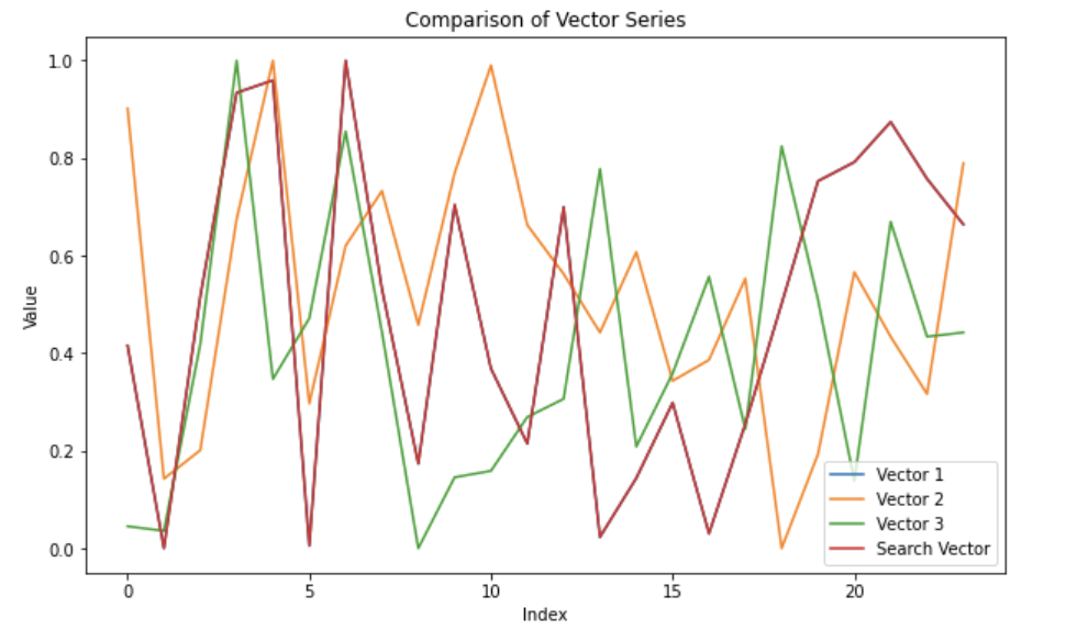
Notice how Vector 1 and Search Vector overlap because the vector with the smallest difference will be the same vector, data_to_insert[1]. We also perform an MAE (mean absolute error) to quantify the similarity. Note that, in this context, the MAE doesn’t hold much meaning because we generated random data. In a real-world example, you would compare time series data representing an event and following a general pattern or behavior. You would also be searching across a lot more data.
# Calculate MAE
mae = np.mean(np.abs(np.array(vectors_to_search[0]) - np.array(data_to_plot[1]["Vectors"])))
print(f"MAE: {mae}")
# A MAE of 0.3 indicates moderate to high dissimilarity which is expected when comparing random data.
MAE: 0.3145208857923114
Final thoughts
I hope this tutorial serves as a boilerplate for combining a time series database—like InfluxDB—and Milvus to identify similar patterns in your time series data.
Get started with InfluxDB Cloud 3.0 here. If you need help, please reach out via our community site or Slack channel.
