Using InfluxDB to Predict The Next Extinction Event

By Mark Herring / Product, Use Cases, Developer
Oct 21, 2019

Navigate to:

An alternative title could be “How to get JSON into InfluxDB Cloud 2.0” but that sounded too boring!

OK, maybe the title is a bit of a stretch goal, but I wanted to take my new InfluxDB Cloud account to ingest some real data (I chose Meteorites, hence the title), and see how quickly I could visualize the data. Full disclosure I had not tried this before!

I have broken this blog post into two major sections:

Section 1: The time to awesome approach
Section 2: The step-by-step reality

Section 1: The time to awesome approach

Like one of those cooking shows, here are some ingredients…Tada here is the cake…

Step 1 – Find the data

I looked for some interesting data sets and settled on the Earth Meteorite Landings. Why? I wanted to predict the end of the world what better way than a Meteorite takes out the earth. Hey maybe that should be a movie…Oh yeah, been there done that.

The data:

 {
  "name": "Aachen",
  "id": "1",
  "nametype": "Valid",
  "recclass": "L5",
  "mass": "21",
  "fall": "Fell",
  "year": "1880-01-01T00:00:00.000",
  "reclat": "50.775000",
  "reclong": "6.083330",
  "geolocation": {
  "type": "Point",
  "coordinates": [
6.08333,
50.775
  ]
    }
       },

Step 2 – Use Telegraf to parse the JSON

Next step — configure Telegraf to connect to the dataset and extract the interesting data. Here is a snippet of my Telegraf configuration file:

[[inputs.http]]
  interval = "10s"

  ## One or more URLs from which to read formatted metrics
  urls = [
    "https://data.nasa.gov/resource/y77d-th95.json"
  ]

  name_override = "meteorevent"

  tagexclude = ["url"]

  ## HTTP method
  method = "GET"
## Tag keys is an array of keys that should be added as tags.
      tag_keys = [
    "recclass"

  ]

  ## String fields is an array of keys that should be added as string fields.

  ## String fields is an array of keys that should be added as string fields.
  json_string_fields = [
      "fall",
    "name",
    "mass"]

  ## Name key is the key to use as the measurement name.
  json_name_key = ""

  ## Time key is the key containing the time that should be used to create the
  ## metric.
  json_time_key = "year"

  ## Time format is the time layout that should be used to interprete the json_time_key.
  ## The time must be `unix`, `unix_ms`, `unix_us`, `unix_ns`, or a time in the
  ## "reference time".  To define a different format, arrange the values from
  ## the "reference time" in the example to match the format you will be
  ## using.  For more information on the "reference time", visit
  ## https://golang.org/pkg/time/#Time.Format
  ##   ex: json_time_format = "Mon Jan 2 15:04:05 -0700 MST 2006"
  ##       json_time_format = "2006-01-02T15:04:05Z07:00"
  ##       json_time_format = "01/02/2006 15:04:05"
  ##       json_time_format = "unix"
  ##       json_time_format = "unix_ms"

json_time_format = "2006-01-02T15:04:05.000"

  ## Timezone allows you to provide an override for timestamps that
  ## don't already include an offset
  ## e.g. 04/06/2016 12:41:45
  ##
  ## Default: "" which renders UTC
  ## Options are as follows:
  ##   1. Local               -- interpret based on machine localtime
  ##   2. "America/New_York"  -- Unix TZ values like those found in https://en.wikipedia.org/wiki/List_of_tz_database_time_zones
  ##   3. UTC                 -- or blank/unspecified, will return timestamp in UTC
  #json_timezone = ""

  [[processors.converter]]
  [processors.converter.fields]
   integer = ["mass"]

Step 3 – Use Telegraf to send the data to InfluxDB Cloud

Set your token, put in the organization and the bucket you want to land the data in:

[[outputs.influxdb_v2]]	
  ## The URLs of the InfluxDB cluster nodes.
  ##
  ## Multiple URLs can be specified for a single cluster, only ONE of the
  ## urls will be written to each interval.
  ## urls exp: http://127.0.0.1:9999
  urls = ["https://PUT IN YOUR URL.influxdata.com"]

  ## Token for authentication.
  token = "$INFLUX_TOKEN"

  ## Organization is the name of the organization you wish to write to; must exist.
  organization = "PUT IN YOUR ORGANIZATION"

  ## Destination bucket to write into.
  bucket = "Meteroite3"

Then just spin up telegraf:

telegraf --config mytelegraf.conf

Step 4 – Visualize the data

Log into InfluxDB Cloud, and build a query:

from(bucket: "Meteroite3")
  |> range(start: -100y)
  |> filter(fn: (r) => r._field == "mass")
  |> group()
  |> aggregateWindow(every: 1y, fn: count, createEmpty: false)

And show the results.

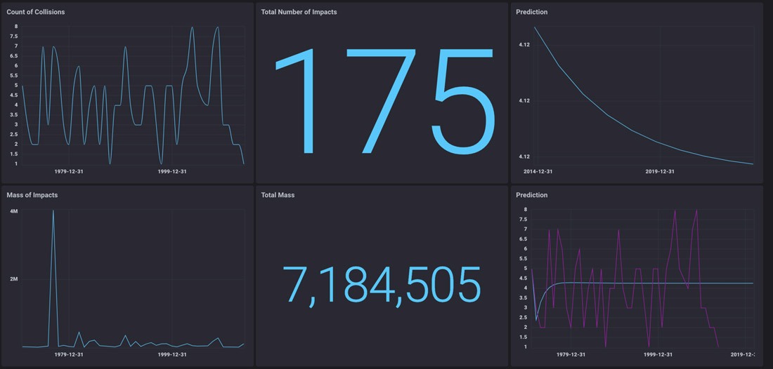
Wow, wasn’t that easy!

Section 2: The step-by-step reality

I decided to also tell you what my journey was really like. I am hoping that the journey will help others on their journey because the platform wasn’t as easy as I had read in that awesome marketing literature, but I know next time it will be much easier.

Step 0 – Create a Cloud 2.0 account

This was really simple: I signed up for InfluxDB Cloud, validated my email and logged in. I was inspired by Samantha Wang’s blog but wanted to use “my own” dataset. I chose the dataset as described above and was ready to go.

Step 1 – Configure Telegraf

Installing Telegraf was pretty easy, the Docs were pretty clear, and it was running in no time. Now all I needed to do was to configure it! Back to Cloud, to get the data from JSON.

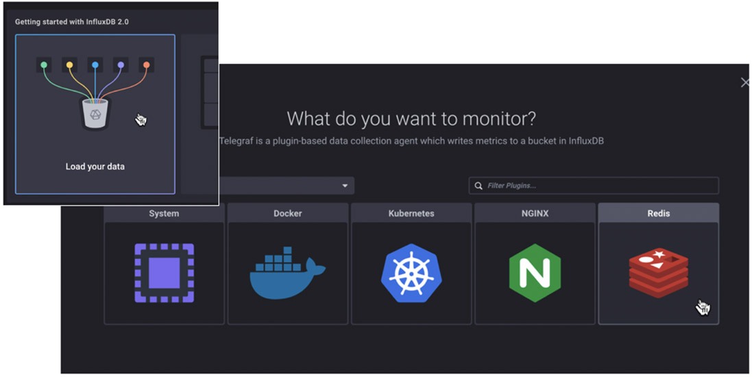
Loved the “Load your data” visualization…But where was “Load from JSON”? Grrr.. back to the Docs, off to GitHub, and now I was getting deeper down the rabbit hole!

On GitHub, I read about the JSON Plugin Parser and created my first configuration file for Telegraf.

[[inputs.file]]
  files = ["example"]

  name_override = "meteorevent"

  tagexclude = ["url"]

  ## HTTP method
  method = "GET"
## Tag keys is an array of keys that should be added as tags.
      tag_keys = [
    "recclass"

  ]

  ## String fields is an array of keys that should be added as string fields.

  ## String fields is an array of keys that should be added as string fields.
  json_string_fields = [
      "fall",
    "name",
    "mass"]

  ## Name key is the key to use as the measurement name.
  json_name_key = ""

  ## Time key is the key containing the time that should be used to create the
  ## metric.
  json_time_key = "year"

  ## Time format is the time layout that should be used to interprete the json_time_key.
  ## The time must be `unix`, `unix_ms`, `unix_us`, `unix_ns`, or a time in the
  ## "reference time".  To define a different format, arrange the values from
  ## the "reference time" in the example to match the format you will be
  ## using.  For more information on the "reference time", visit
  ## https://golang.org/pkg/time/#Time.Format
  ##   ex: json_time_format = "Mon Jan 2 15:04:05 -0700 MST 2006"
  ##       json_time_format = "2006-01-02T15:04:05Z07:00"
  ##       json_time_format = "01/02/2006 15:04:05"
  ##       json_time_format = "unix"
  ##       json_time_format = "unix_ms"

json_time_format = "2006-01-02T15:04:05.000"

  ## Timezone allows you to provide an override for timestamps that
  ## don't already include an offset
  ## e.g. 04/06/2016 12:41:45
  ##
  ## Default: "" which renders UTC
  ## Options are as follows:
  ##   1. Local               -- interpret based on machine localtime
  ##   2. "America/New_York"  -- Unix TZ values like those found in https://en.wikipedia.org/wiki/List_of_tz_database_time_zones
  ##   3. UTC                 -- or blank/unspecified, will return timestamp in UTC
  #json_timezone = ""

Oh no, but I didn’t have a file mine was a URL. I thought about “cheating”, but no, I wanted this to be a “real example” so I find out how to get data from a URL. Updated the top of my config file:

[[inputs.http]]
  interval = "10s"

  ## One or more URLs from which to read formatted metrics
  urls = [
    "https://data.nasa.gov/resource/y77d-th95.json"
  ]

Fantastic! Got data coming in (I hope). Oh, how do I tell it to go to my Cloud instance? Back to the Docs, where I found out about manually configuring Telegraf.

[[outputs.influxdb_v2]]
  urls = ["put in your URL"]
  token = "$INFLUX_TOKEN"
  organization = "orgname"
  bucket = "example-bucket"

Back to Cloud, created my bucket, created my token. OK, I was seriously ready.

Fire up telegraf:

telegraf --config mytelegraf.conf

And

ERROR:
Error in plugin: [url=https://data.nasa.gov/resource/y77d-th95.json]: parsing time "1880-01-01T00:00:00.000" as "unix": cannot parse "1880-01-01T00:00:00.000" as "unix"

Ok so I knew that my

json_time_format = "2006-01-02T15:04:05Z07:00"

was wrong, but what should it be? From the JSON, I could see it was:

"year": "1880-01-01T00:00:00.000",

But what to change json_time_format = "2006-01-02T15:04:05Z07:00" to be?

I think I tried everything…So I “phoned a friend”, David McKay, the exceptional DevRel who happens to be just a Slack message away. He comes back with:

json_time_format = "2006-01-02T15:04:05.000"

OK, I have no idea how he got that…Don’t see it in the Docs, but other than being amazed at how good he was, I was eager to continueHe also gave me one more bit of advice for my config file.

[[processors.converter]]
 [processors.converter.fields]
   integer = ["mass"]
   float = ["reclat", "reclong"]

I updated my config…let’s go!

Darn, another error:

[inputs.http]: Error in plugin: [url=https://data.nasa.gov/resource/y77d-th95.json]: JSON time key could not be found

Checked Cloud…No data! Grrrrrr.

OK, I was so close… What to do? I thought for a short second of giving up – nope I was not going to do that! It was time to “call another friend” – (side note, why not call David again? Well, I thought if I send my requests in parallel across the org, no one would understand how “needy” I was). But I am a sucker for punishment, so it is all revealed in this blog! Russ Savage to the rescue (Russ is the Director of Product Management at InfluxData). He found that in the JSON, there were a few entries with no year value. Another learning experience for me — if Telegraf finds an error in JSON, it just stops…Nothing is written!

So what to do? Ok I cheated…I copied the JSON file, removed the offending entries, saved it and went back to:

[[inputs.file]]
  files = ["mynewdata.JSON"]

Step 2 – Get data in...

Success…Telegraf got the data from JSON to Cloud 2.0. I then killed the telegraf process after 15 seconds. No need to run the same file again and again. Also got a few issues logged against Telegraf.

Step 3 – Visualize the data

This was almost the easiest part. I say “almost” because I first tried Data Explorer.

Newbie tip: Set time to be much longer than last hour! My data was old!

Changing that and wow…I have data!

What I did learn is that Data Explorer was good but maybe too smart for me.

from(bucket: "Meteroite3")
  |> range(start: v.timeRangeStart, stop: v.timeRangeStop)
  |> filter(fn: (r) => r._measurement == "file")
  |> filter(fn: (r) => r._field == "mass")
  |> aggregateWindow(every: v.windowPeriod, fn: sum)
  |> yield(name: "sum")

I simplified this script to:

from(bucket: "Meteroite3")
  |> range(start: -100y)
  |> filter(fn: (r) => r._field == "mass")
  |> group()
  |> aggregateWindow(every: 1y, fn: sum, createEmpty: false)

Step 4 – Predict the future!

Ok, so I decided to use Holt-Winters to predict the future:

from(bucket: "Meteroite3")
|> range(start: -100y, stop:-8y)
|> filter(fn: (r) => r._field == "mass")
|> group()
|> aggregateWindow(every: 1y, fn: count, createEmpty: false)
|> holtWinters(n: 10, seasonality: 0, interval: 1y, withFit: true)
|> yield(name:"prediction")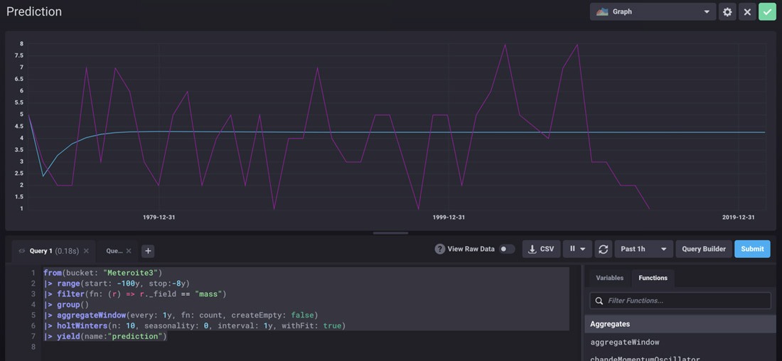

So it shows we will all live…Don’t worry!

I did speak to our ML expert, and this is what she said:

"In order to use Triple Exponential Smoothing (Holt-Winters) or Double Exponential Smoothing, your data needs to exhibit trend and seasonality or just trend, respectively. Your data doesn't have any clear seasonality or trend." – Anais Dotis-Georgiou

Thanks to everyone who helped me predict the next extinction event!

Navigate to:

Try InfluxDB Cloud

Stop flying blind

Using InfluxDB to Predict The Next Extinction Event

By Mark Herring / Product, Use Cases, Developer
Oct 21, 2019

Navigate to:

Section 1: The time to awesome approach

Step 1 – Find the data

Step 2 – Use Telegraf to parse the JSON

Step 3 – Use Telegraf to send the data to InfluxDB Cloud

Step 4 – Visualize the data

Section 2: The step-by-step reality

Step 0 – Create a Cloud 2.0 account

Step 1 – Configure Telegraf

Step 2 – Get data in...

Step 3 – Visualize the data

Step 4 – Predict the future!

Try InfluxDB Cloud

Learn more about InfluxDB

Performance Benchmarking: InfluxDB 3.0 vs. InfluxDB Open Source

InfluxDB for Industrial IoT:  
A Live Demonstration

How Time Series Databases and Data Lakes Work Together

Data Warehousing

Network Monitoring

Time Series Data Analysis: Definitions and Best Techniques in 2024

Platform

Integrations

Navigate to:

Try InfluxDB Cloud

Stop flying blind

Get Updates

Using InfluxDB to Predict The Next Extinction Event

By Mark Herring / Product, Use Cases, Developer Oct 21, 2019

Navigate to:

Section 1: The time to awesome approach

Step 1 – Find the data

Step 2 – Use Telegraf to parse the JSON

Step 3 – Use Telegraf to send the data to InfluxDB Cloud

Step 4 – Visualize the data

Section 2: The step-by-step reality

Step 0 – Create a Cloud 2.0 account

Step 1 – Configure Telegraf

Step 2 – Get data in...

Step 3 – Visualize the data

Step 4 – Predict the future!

Try InfluxDB Cloud

Learn more about InfluxDB

Performance Benchmarking: InfluxDB 3.0 vs. InfluxDB Open Source

InfluxDB for Industrial IoT: A Live Demonstration

How Time Series Databases and Data Lakes Work Together

Data Warehousing

Network Monitoring

Time Series Data Analysis: Definitions and Best Techniques in 2024

By Mark Herring / Product, Use Cases, Developer
Oct 21, 2019

InfluxDB for Industrial IoT:  
A Live Demonstration