Build a Home Internet Speed Test with Grafana and InfluxDB

By Jessica Wachtel / Product
Oct 04, 2023

This post was originally published on The New Stack and is reposted here with permission.

A tutorial on how to use time series data to test your home internet speeds.

Time series data is ubiquitous in everyday life. Collecting, storing and analyzing time series data provides clarity and insight on just about anything. Time series data exists in outer space and inside your home. Time series data also sheds light on the dark question: “Am I getting the internet speeds I’m paying for?” Rather than write another article about how InfluxDB can turn time series data into real-time insights, this tutorial shows you how to track your internet speeds and to finally answer your questions about whether your internet really is too slow or if you might need to do a bit of deeper breathing.

This tutorial uses the TIG stack which includes Telegraf, InfluxDB Cloud Serverless and Grafana. For detailed information about this “TIG” stack, check out this article. The time series data in this tutorial comes directly from your home internet. Telegraf’s Home Internet Speed Plugin will collect the data. The Home Internet Speed Plugin uses Speedtest by Ookla to test a user’s internet speed and quality. The test locates the closest servers, finds the best latency, then downloads and uploads a file from the selected server to capture the user’s internet connection speed.

Required materials

Before getting started, make sure you have the following:

• Free InfluxDB Cloud Serverless Account
• Free Grafana cloud account
• Telegraf installed on your machine

Part one: InfluxDB Cloud Serverless

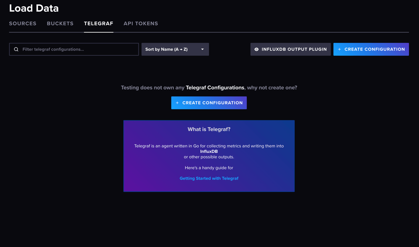
Login to InfluxDB Cloud Serverless and go to the Resource Center, navigate to “Add Data” and select “Configure Agent”. This takes you to the Telegraf section. Then select “Create Configuration”:

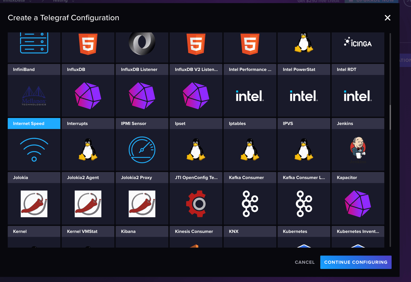
Use the “Bucket” dropdown to select an existing bucket or create a new one. Then scroll down through the Telegraf plugins until you reach the “Internet Speed” plugin. Click the “Internet Speed” plugin followed by the “Continue Configuring” blue button that appears in the bottom right-hand corner.

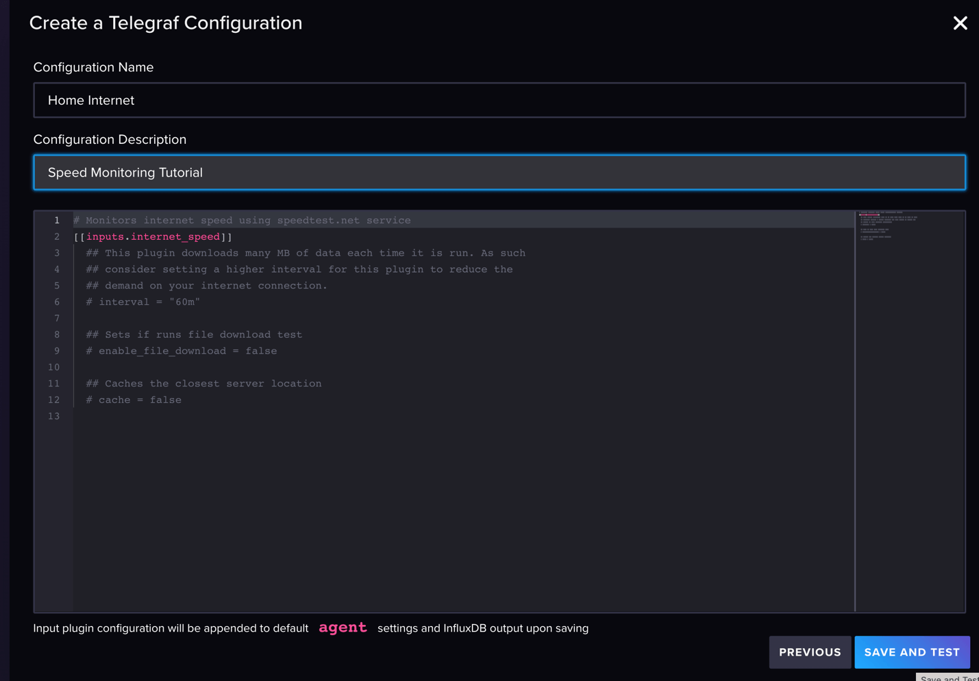
Name the configuration. You can add a brief description if you want. Complete this section by selecting “Save and Test”:

Next, open your terminal. If you don’t already have an API token for your bucket, create one at the API Token tab. Once you have a token with the settings you want, copy the API token and paste it into the terminal and save it to a text pad page. This token will disappear as soon as you leave this page so it’s important to save it. Copy the “Start Telegraf” command and paste that into the text pad.

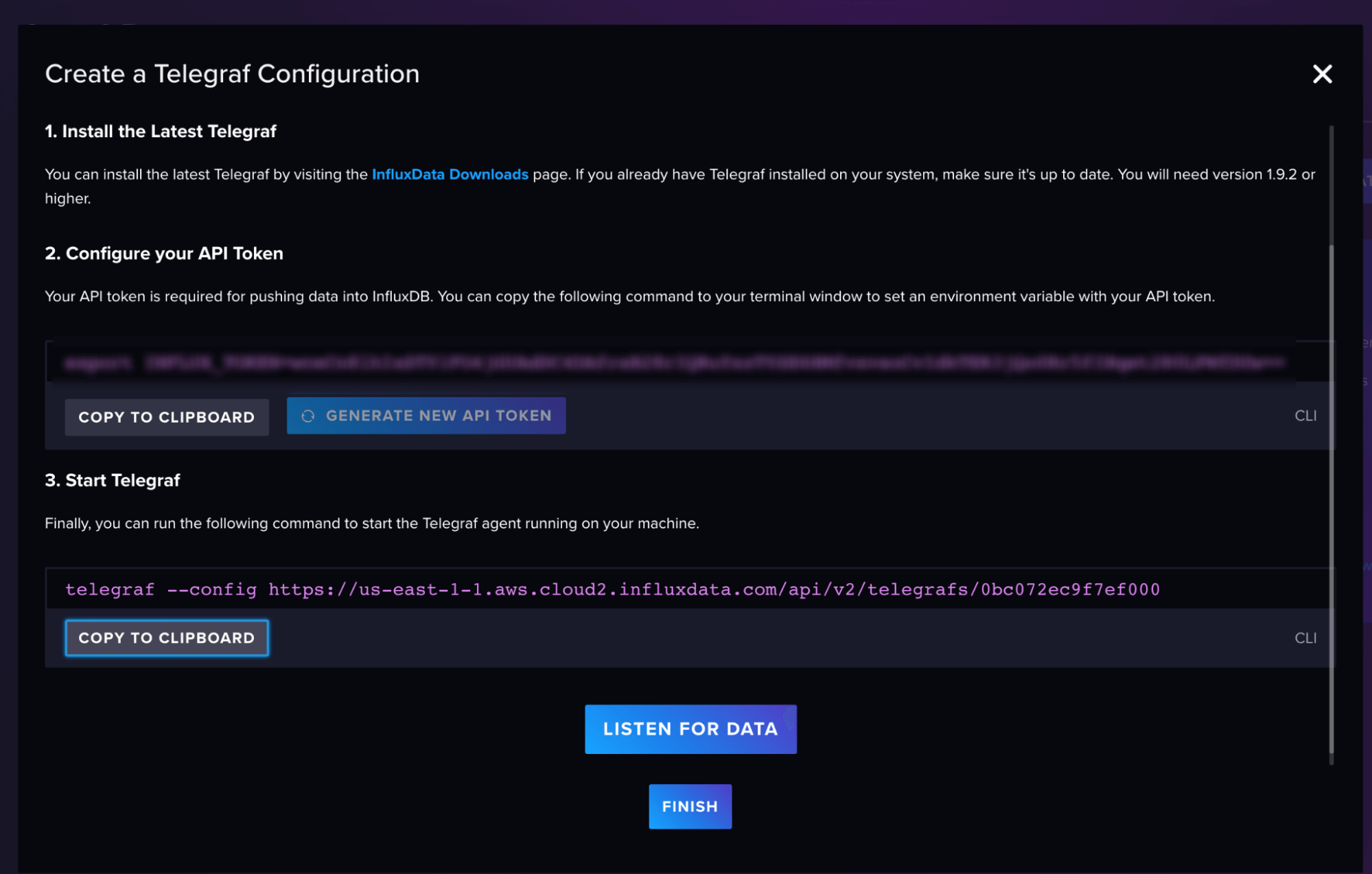
Click “Finish” to close the window.

As soon as the “Create a Telegraf Configuration” window closes, you’ll see the name of the Telegraf configuration you just created appear on the main section of your screen. Click on the name of that configuration. Just below [agent] you’ll see interval = “20s”, so update that to interval = “60s”. This gives Telegraf a longer window to gather data from the speed test servers.

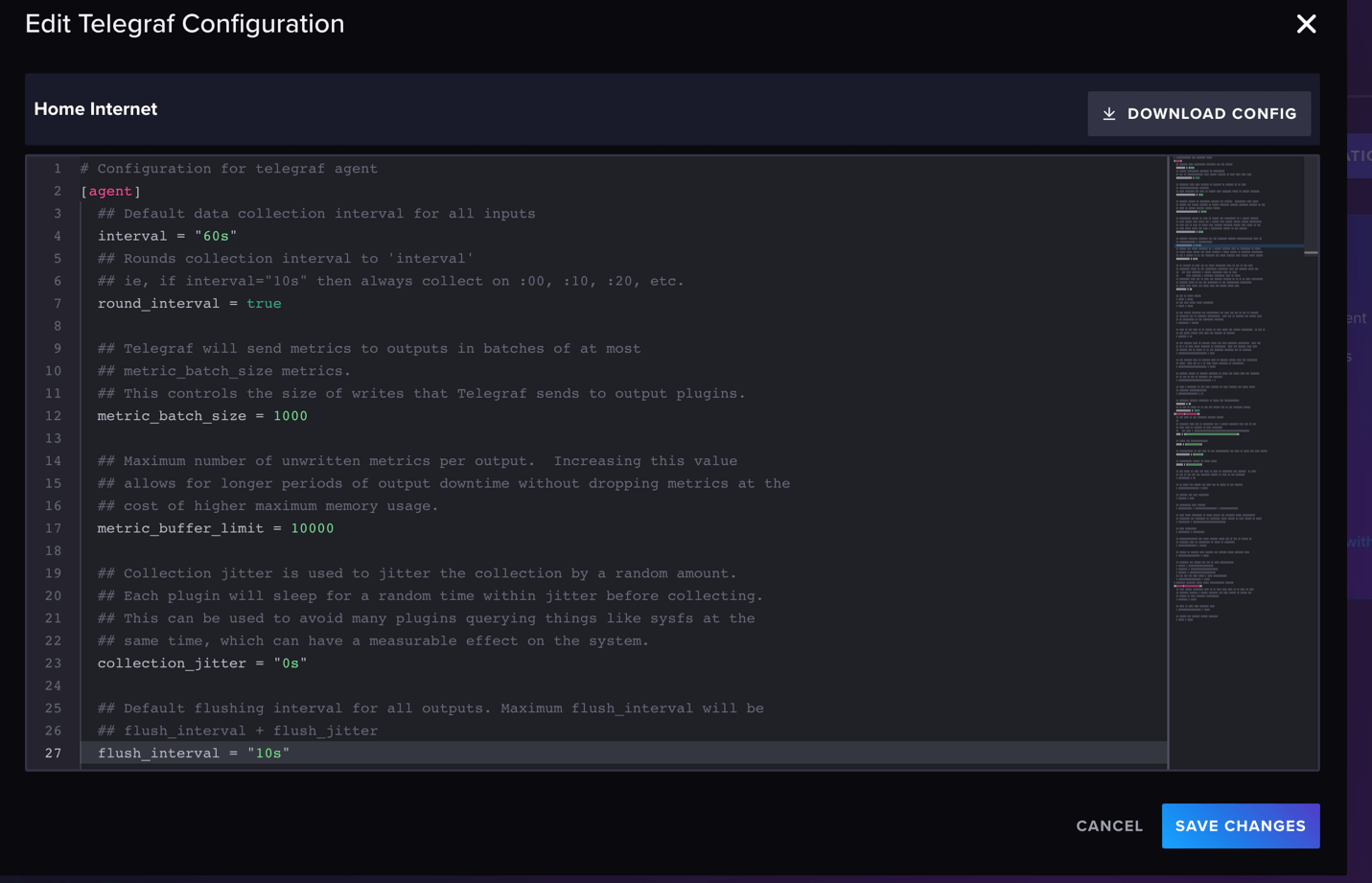
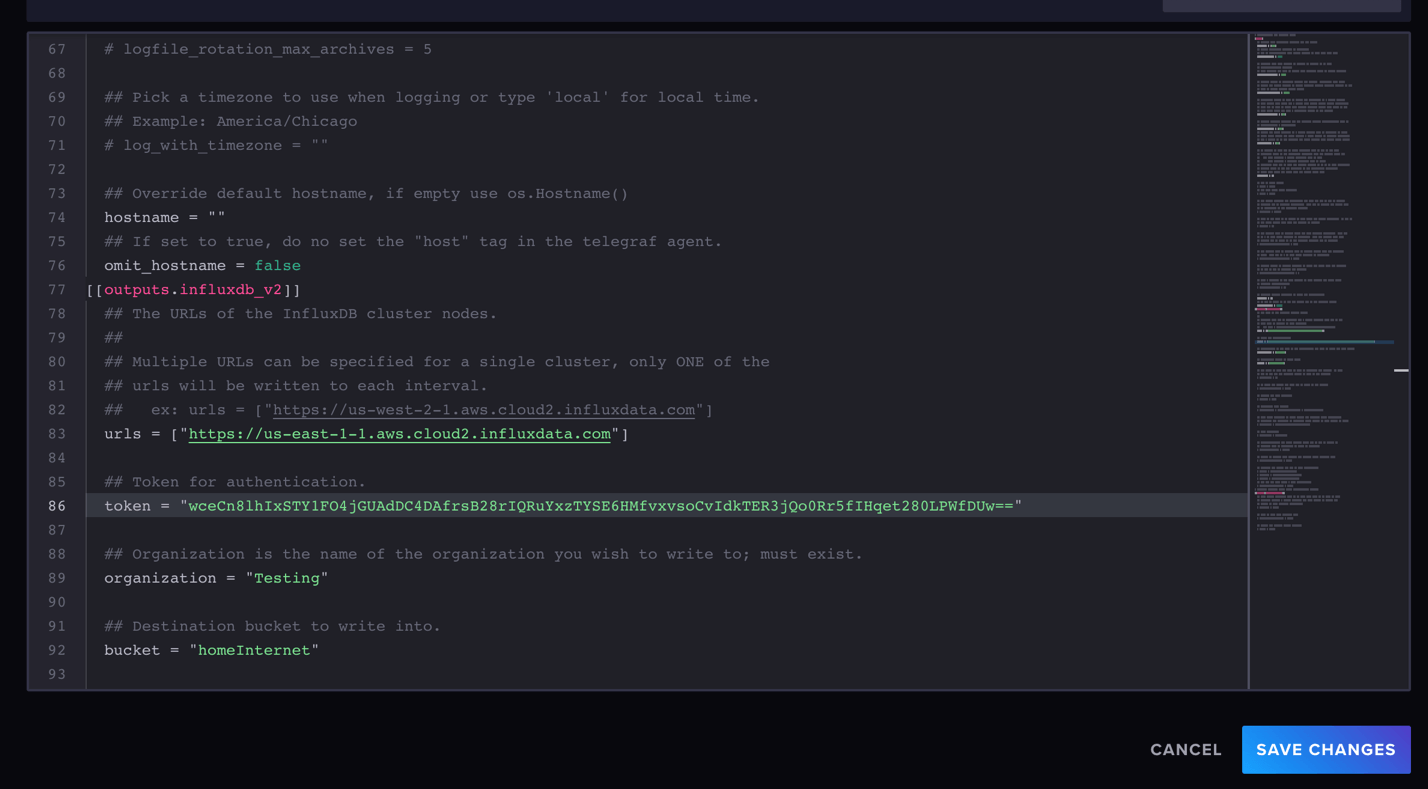
Locate the line that contains token = $INFLUX_TOKEN and replace the $INFLUX_TOKEN value with the API token you copied earlier. Complete this step by selecting “Save Changes”:

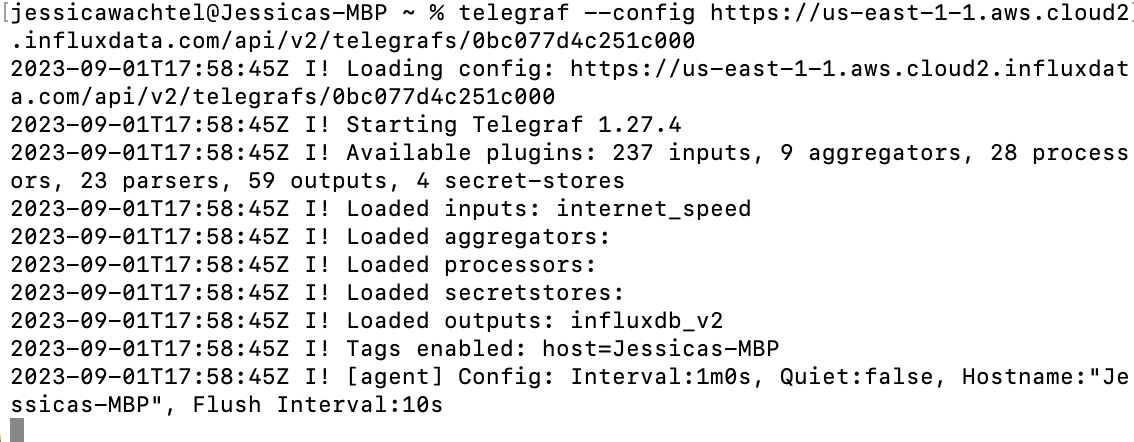
Paste the entire “Start Telegraf” command from your text pad into your terminal. The command includes telegraf -- config + URL This is the only command needed to start Telegraf. The image below depicts what a successfully started Telegraf instance looks like:

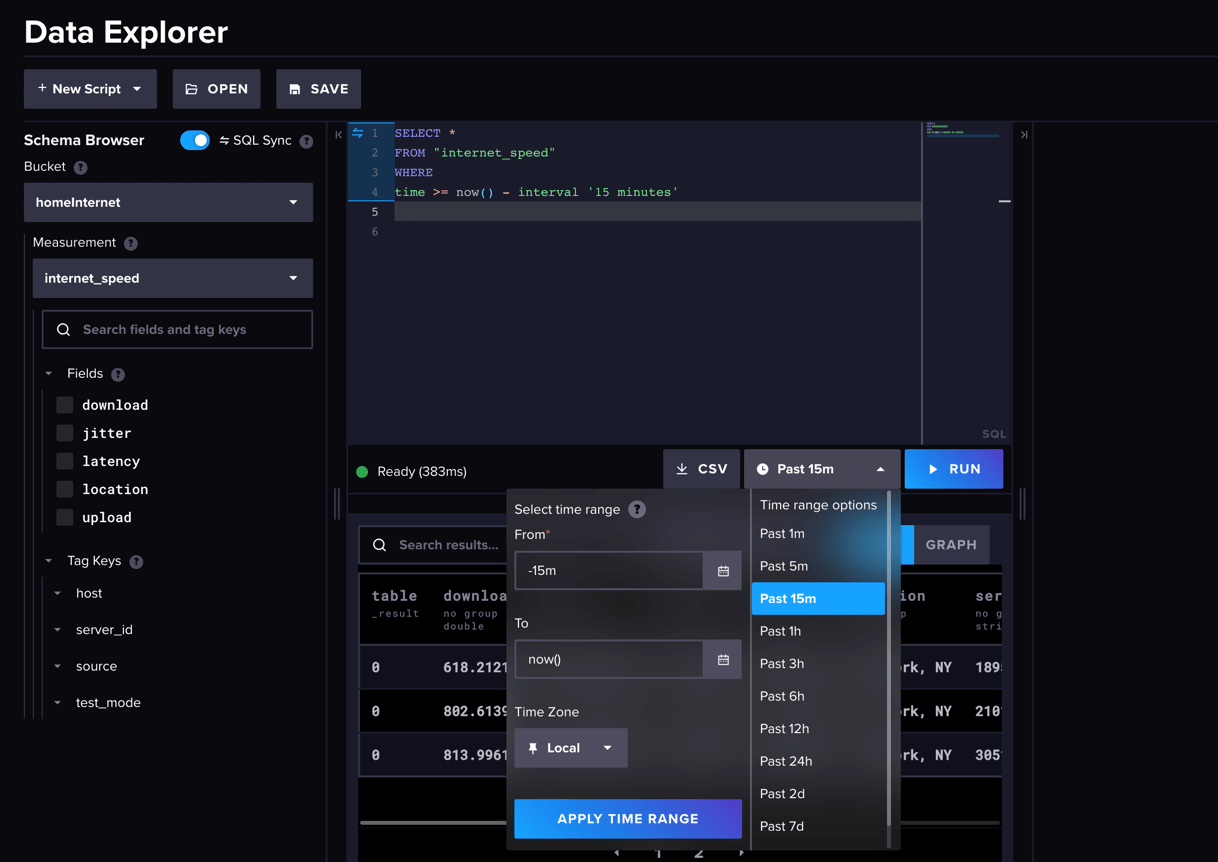
The last thing to do in Part One is watch the data appear. Head to the Data Explorer (the graph icon on the top left side of the page). You can immediately query the data using SQL. You can organize the query by fields or tags. The Data Explorer includes a dropdown menu UI, meaning you don’t need to have deep SQL knowledge to execute queries.

Part two: Configuring and visualizing data with Grafana

Part Two follows along with this tutorial, which also includes a YouTube video component.

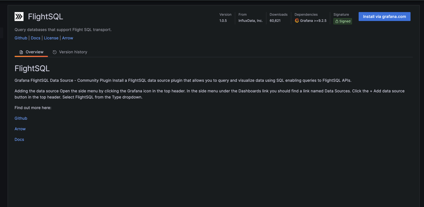
Launch Grafana Cloud. Click “Connect Data” in the top right-hand corner. Select FlightSQL and select “Add New Data Source” in the top right-hand corner. Select “install via Grafana.com” to install FlightSQL:

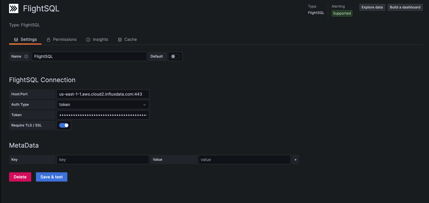
Click on settings in the FlightSQL Plugin. The host name comes from InfluxDB Cloud Serverless. The host name is the URL with the protocol omitted.

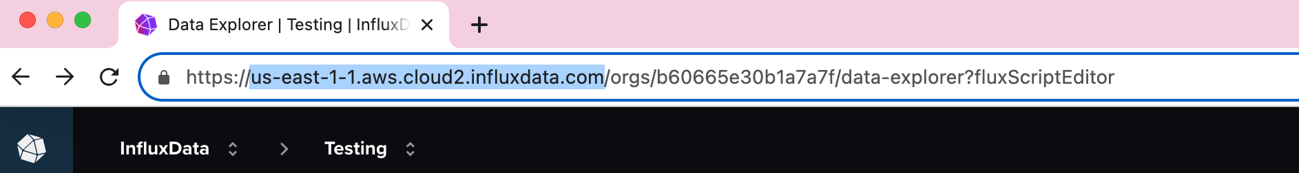
For the port, define the secure port 443. The entire Host:Port will end up looking similar to this:

us-east-1-1.aws.cloud2.influxdata.com:443

The next step is to define the authentication type. Select “token” from the dropdown menu because InfluxDB Cloud Serverless uses tokens. Navigate back to InfluxDB Cloud Serverless because InfluxDB generates the token.

In InfluxDB Cloud Serverless’s main menu, navigate to Access Token Manager > Go to Tokens. Select Generate API Token > All Access API Token. Write a description if desired and save. Copy the token because it will disappear once you close the window. Navigate back to Grafana.

Once in Grafana, paste the all-access token into the text box. Then enable TLS/ SSL. This completes the basic connection setup.

The final setup step is enabling metadata. The metadata defines exactly where to query within InfluxDB Cloud Serverless. We query by bucket which is essentially its own database within InfluxDB. We’ll use the key “bucket-name” and the value will be the same as the bucket name that the home internet data is being sent.

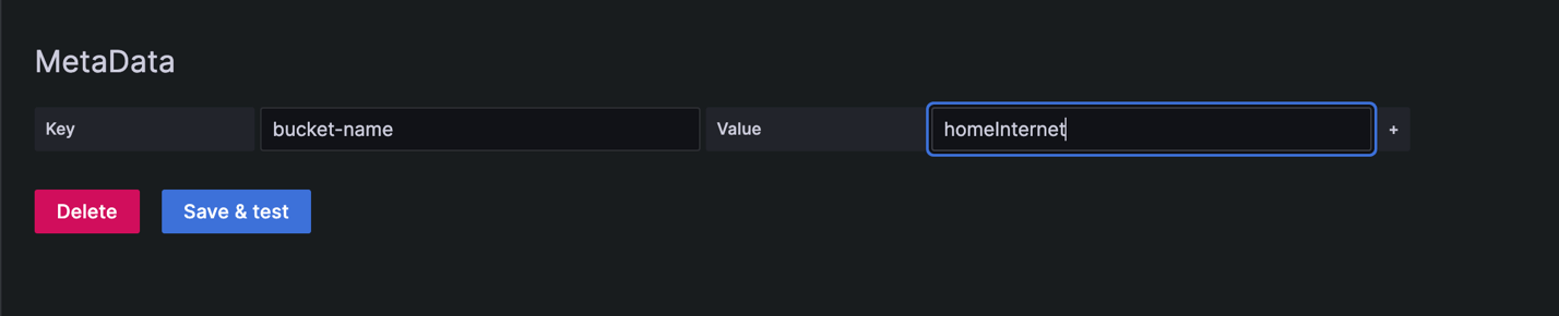
When you’re done, click Save & Test. If everything was set up correctly, the OK message will appear.

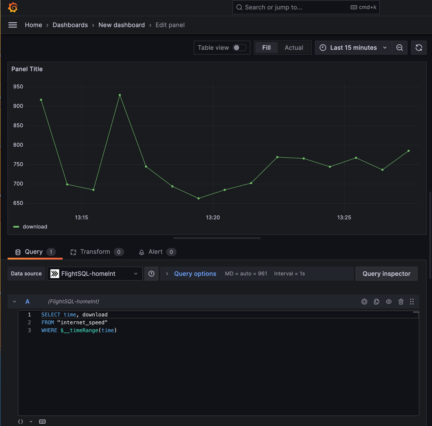
The next step in our Grafana configuration is building the dashboard. Navigate to the dashboard panel and create a new dashboard. Select “Add New Panel”. Once the new window opens you’ll be able to see the FlightSQL data source just above the SQL editor around the middle of the page. Grafana helps generate SQL and allows for custom SQL generation. This example uses custom SQL generation. To open the custom SQL editor, click “Edit SQL”.

The custom SQL query we’re going to use is this:

SELECT time, download
FROM "internet_speed"
WHERE $__timeRange(time)

This query selects the time and the download fields from the bucket internet_speed. The $__timeRange(time) means we can update the time range from the dropdown menu. Clicking on the circular arrows to the top right of the panel creates or refreshes the image.

Part three: data analysis

Looking at the graph above, it’s clear that my internet speeds are mostly within the 650-800mbs range. My first step in analysis is determining whether or not external factors are affecting the download speeds. The next thing I’ll do is add the server_id to my query.

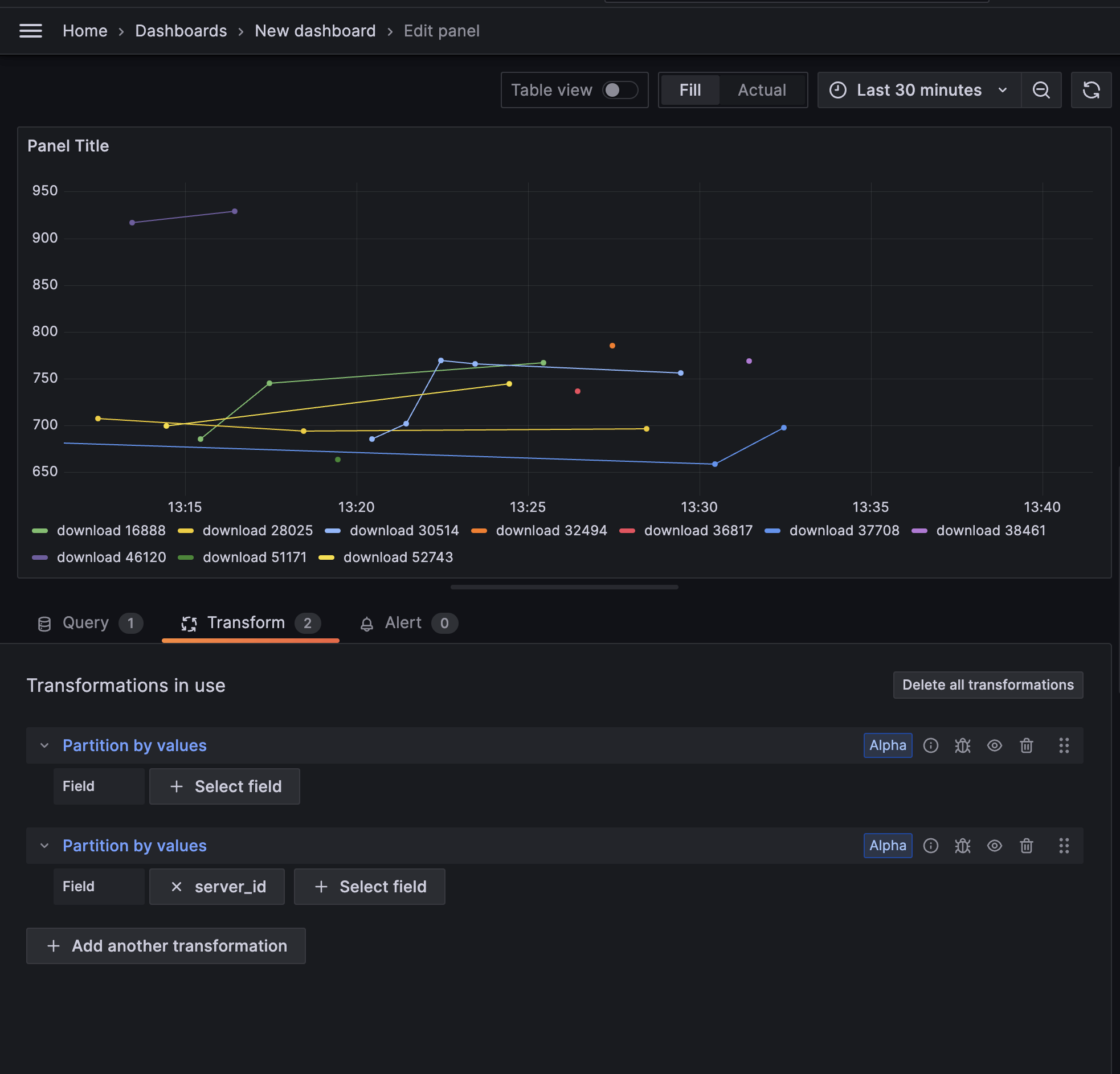
To query by tag, just add the name of the tag in quotes. In this example, the new query line looks like SELECT time, download, "server_id".

Grafana uses a tool called Transformations to organize the results by tag. Click “Transform” and the transformation we’re going to use is “Partition by Values”. Click select field > server_id. The resulting panel now includes each download speed by server id:

This is only the beginning. What other factors are at play? How does the latency affect downloads? What tags and fields do you think matter? Is your internet speed up to par?

Join the time series data revolution

This is just a scratch on the surface of the vast world of time series data. Time series data is everywhere but with the TIG stack, setup never has to be overly complicated and real-time insights are always available.

To keep working within our community, check out our community page which includes a link to our Slack and more cool projects to help get you started.