Finding More Hidden Gems in Holt-Winters

By Anais Dotis-Georgiou / Product, Use Cases, Developer
Mar 07, 2019

Welcome back to this three-part blog post series on Holt-Winters and why it’s still highly relevant today. To understand Part Two, I suggest reading Part One, in which we covered:

1. When to use Holt-Winters;
2. How Single Exponential Smoothing works;
3. A conceptual overview of optimization for Single Exponential Smoothing;
4. Extra: The proof for optimization of Residual Sum of Squares (RSS) for Linear Regression.

In this piece, Part Two, we’ll explore:

1. How Single Exponential Smoothing relates to Triple Exponential Smoothing/Holt-Winters;
2. How RSS relates to Root Mean Square Error (RMSE);
3. How RMSE is optimized for Holt-Winters using the Nelder-Mead method.

In Part Three, we’ll explore:

1. How you can use InfluxDB's built-in Multiplicative Holt-Winters function to generate predictions on your time series data;
2. A list of learning resources.

How Single Exponential Smoothing relates to Triple Exponential Smoothing/Holt-Winters

Like SES, Holt-Winters, which can be employed as a powerful and efficient predictive maintenance technique, determines the forecasted value by calculating an exponentially weighted average – but it doesn’t stop there.

As Holt and Winters have previously written, if your data has a trend and seasonality, then you should calculate a weighted average of those values as well and incorporate them into the forecasted value.

The Holt-Winters’ Multiplicative method looks like this:

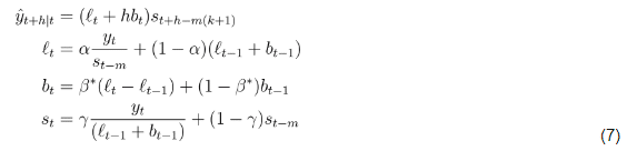
where, l_(t) is the smoothing equation, b_(t) is the slope, and s_(t) is the seasonality. There are two additional smoothing parameters beta-star and gamma for the slope and seasonality, respectively. The number of points that we wish to forecast is denoted by the integer h. The number of seasons in a cycle (usually measured in years, but months or days, depending on your timescale) is represented by m, and k is an index which ensures that forecasts are based on the appropriate season. The forecasted value, y-hat is derived from taking three characteristics of the data into consideration, which is where Triple Exponential Smoothing gets its name. Notice, however, that each equation still bears quite a bit of similarity to SES and is an exponentially weighted mean.

Finally, Equation (7) is the multiplicative method (there is also an Additive Holt-Winters method). The additive approach is used when the seasonal periods are constant. The multiplicative method is used when the seasonal periods are changing proportionally to the level (or slope) of the series. This proportionality is represented by the following portion of the seasonality equation:

I totally agree Holt-Winters looks quite a bit hairier. However, now you can imagine that all we need to do is find three smoothing parameters instead of one and some more initial values. This optimization is performed in the same way that we did linear regression optimization. The only difference is that we can’t just take a partial derivative to find the smoothing factors; instead, we will use the Nelder-Mead method. And rather than optimizing the RSS, we will optimize the RSME instead. “Why?” do you ask?

How RSS relates to RMSE

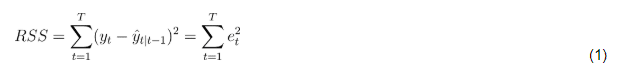
RMSE is used for two main reasons: 1) it is scale-dependent, and 2) it is normalized. RMSE is scale-dependent because the errors are expressed in the same units as y_(t). Since the errors are on the same scale, they make intuitive sense. By contrast, with RSS, the errors are squared. RMSE is also normalized, while SSE is more variable and dependent on the sample size.

As a reminder, RSS looks like this:

While RMSE is merely,

In other words, RMSE is the square of RSS divided by the number of degrees of freedom.

How RMSE is optimized for Holt-Winters using the Nelder-Mead Method

Remember that bowl that we made for the minimization of RSS? In order to find one smoothing parameter (alpha) and one initial value (l_nought)? Well, now we also have to find two more smoothing parameters (beta-star and gamma) and one more initial value (b_nought). Our optimization has evolved from a three-dimensional problem to a six-dimensional one. We would have to execute some pretty hard differential equations to solve it. We no longer have a pretty bowl either. There are local minima as well as global minima. As a result, we can’t merely set the partial derivatives equal to 0 and solve for these parameters. Instead, we have to use a more sophisticated method:  the Nelder-Mead method. The Nelder-Mead is a numerical method, an approximation, a mathematical tool or a shortcut to solving difficult math problems.

The Nelder-Mead method is not a true global optimization algorithm. However, it works pretty well for problems that do not have many local minima, such as ours. It works by placing a simplex, in space. This simplex is like a little amoeba or animated glob. However, it can only move downhill. It stretches a little bit in each direction to determine where the downhill is. Once it’s found it, it moves a little downhill. It repeats the process until it can’t move anymore. At this point, the simplex is “happy” and we’ve found our minimum. The shape and position of the simplex are determined by the method. The wiggling of the simplex downhill is just carried out by a series of operations applied to it in a for loop, i.e. iteratively. The benefit of using numerical methods for optimizations is that we can find really good approximations by using simple math instead of trying to perform costly and complicated algebraic computations.

Once we’ve found our minimum, then we have found our smoothing parameters and initial values. We have all the missing pieces in our 3 equations, and we can use Holt-Winters to make predictions.

I hope this tutorial helps get you started on your forecasting journey. If you have any questions, please post them on the community site or tweet us @InfluxDB. As always, here is a brain break: