Getting Started with Python and Geo-Temporal Analysis

By Susannah Brodnitz / Product
Oct 31, 2022

This article was originally published in The New Stack and is reposted here with permission.

Working with geo-temporal data can be difficult. In addition to the challenges often associated with time-series analysis, like large volumes of data that you want real-time access to, working with latitude and longitude often involves trigonometry because you have to account for the curvature of the Earth. That’s computationally expensive. It can drive costs up and slow down programs. Fortunately, InfluxDB’s geo-temporal package is designed to handle these problems.

The package does this with S2 geometry. The S2 system divides the Earth into cells to help computers calculate locations faster. Unlike a lot of other projections, it’s based on a sphere instead of a flat surface, so there are no gaps or overlapping areas. You can choose different levels to vary the size of each cell. With this system, a computer can check how many cells away two points are to get an estimate of their distance.

In a lot of cases, the estimates you can get from S2 calculations are precise enough and much faster for computers than trigonometry. In cases where you need exact answers, using S2 geometry can still speed things up because computers can get rough estimates first and then do only the expensive calculations that are truly needed.

Getting started with an example

For this example, we’re going to calculate the average surface temperature of the ocean over a specified region and at different time windows, as well as the standard deviation. We’re going to be working in InfluxDB’s Python client library in a Jupyter notebook. Here are some other blog posts on these topics.

I used Jupyter notebooks through Anaconda, so the first step for me was to install InfluxDB in Anaconda by typing the following in the command window.

conda install -c conda-forge influxdb

Then, as prompted, I had to update anaconda with

conda update -n base -c defaults conda

The file used in this example is in NetCDF format, so I also had to install the following to read it

conda install -c conda-forge netcdf4

NetCDF files are a common format for scientific data. The data used in this example is the Roemmich-Gilson Argo temperature climatology, which is available here from the second link on the page entitled “2004-2018 RG Argo Temperature Climatology.” This data comes from measurements made by thousands of floats throughout the ocean taking measurements at irregular times and in irregular locations, which are averaged into a gridded product with monthly values on a 1° grid.

In your Jupyter notebook, start by running the following commands to import various packages needed for this example.

import matplotlib.pyplot as plt
import numpy as np
import datetime
import pandas as pd
import influxdb_client, os, time
from influxdb_client import InfluxDBClient, Point, WritePrecision, WriteOptions
from influxdb_client.client.write_api import SYNCHRONOUS
import netCDF4 as nc

Cleaning up the data

Run the following commands to read the file.

file_name = '/filepath/RG_ArgoClim_Temperature_2019.nc'
data_structure = nc.Dataset(file_name)

If you run

print(data_structure.variables.keys())

Then the following should be the output.

dict_keys(['LONGITUDE', 'LATITUDE', 'PRESSURE', 'TIME', 'ARGO_TEMPERATURE_MEAN', 'ARGO_TEMPERATURE_ANOMALY', 'BATHYMETRY_MASK', 'MAPPING_MASK'])

These are the various arrays within the file, which store the data. The ones we’re interested in are LONGITUDE, LATITUDE, TIME, ARGO_TEMPERATURE_MEAN, and ARGO_TEMPERATURE_ANOMALY. To read the data from the file run

lon = data_structure.variables['LONGITUDE']
lat = data_structure.variables['LATITUDE']
time = data_structure.variables['TIME']
temp_mean = data_structure.variables['ARGO_TEMPERATURE_MEAN']
temp_anom = data_structure.variables['ARGO_TEMPERATURE_ANOMALY']

To see the dimensions of each array, run

print(lon.shape)
print(lat.shape)
print(time.shape)
print(temp_mean.shape)
print(temp_anom.shape)

You should see

(360,)
(145,)
(180,)
(58, 145, 360)
(180, 58, 145, 360)

There are 360 longitude values, 145 latitude values and 180 time values. There are also 58 pressure values. Since we’re only interested in the ocean temperature at the surface, which is the lowest pressure, we’re going to subset the array to take the first pressure index.

You will also notice that the mean temperature doesn’t have a time dimension. This dataset separates out temperature into the mean value over the whole time series and the monthly differences from the mean, called anomalies. To get the actual temperature for each month, we just add the mean and anomaly.

If you try to display the value of a random point within the array, you should see

temp_anom[0,0,0,0]

masked_array(data=1.082,
             mask=False,
       fill_value=1e+20,
            dtype=float32)

Right now, each value is within an array as an artifact of being within a netCDF file. Run the following to get simple arrays of values:

lon = lon[:]
lat = lat[:]
time = time[:]
temp_mean = temp_mean[:]
temp_anom = temp_anom[:]

temp_anom[0,0,0,0]

1.082

The unit of time is the number of months since the start of the dataset. To make an understandable date-time vector, run the following.

time_pass=pd.date_range(start='1/1/2004', periods=180, freq='MS')

To create an array of the temperature just at the surface, add together the mean and anomaly arrays at the first pressure index with the following code.

ocean_surface_temp=np.empty((180,145,360))
for itime in range(180):
ocean_surface_temp[itime,:,:]=temp_mean[0,:,:]+temp_anom[itime,0,:,:]

Writing data to InfluxDB Cloud

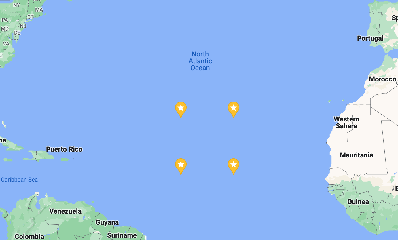
Now that the data we want is in a nicely formatted array, we can get started sending it to InfluxDB Cloud. To save storage space, for this example we’re not going to upload the whole thing, just 10 years of data from a 10-degree-by-10-degree box in the Atlantic Ocean. The coordinates I picked for this are 15.5°N to 25.5°N and 34.5°W to 44.5°W, or latitude indices 80 to 90 and longitude indices 295 to 305.

To send data to InfluxDB most efficiently, we’re going to create an array of data points. We’re going to call each point ocean_temperature, and that name will be set as its measurement.

To use the geo-temporal package in InfluxDB, you need to send in your data with latitude and longitude as fields, so each of our points will have latitude, longitude and temperature fields. In InfluxDB, if there are two field values at the same time stamp, the next value you upload will overwrite the previous one. This is a problem for us because our data has many values for latitude, longitude and temperature at the same time.

A simple way to prevent data from being overwritten is by giving each point a location tag. In our data, there are many measurements at the same time but no two at the same location and time. You can develop other unique tags for points at the same time you don’t want to be overwritten, as described in more detail here.

points_to_send = []
for itime in range(120):
    for ilat in range(80, 90):
        for ilon in range(295, 305):
            p = Point("ocean_temperature")
            p.tag("location", str(lat[ilat]) + str(lon[ilon]))
            p.field("lat", lat[ilat])
            p.field('lon', lon[ilon])
            p.field('temp', ocean_surface_temp[itime,ilat,ilon])
            p.time(time_pass[itime])
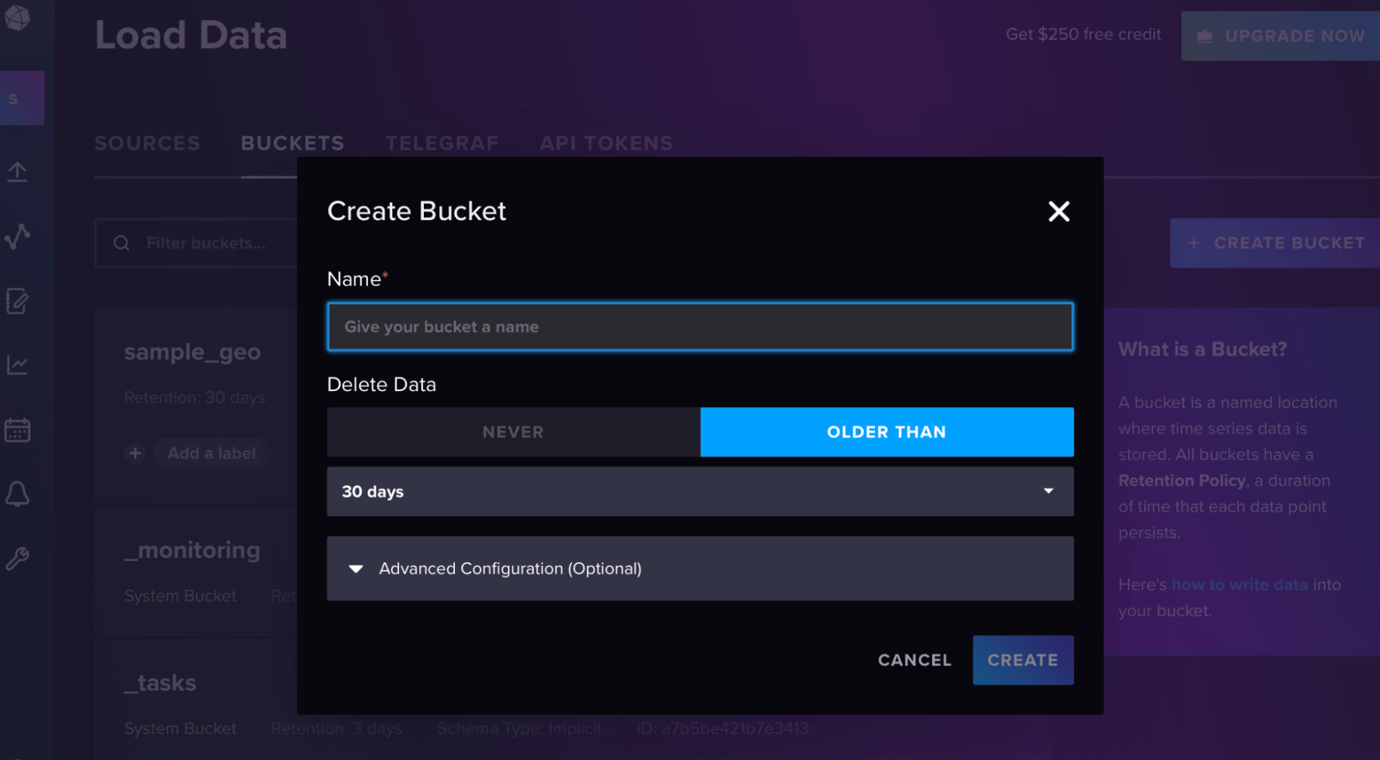
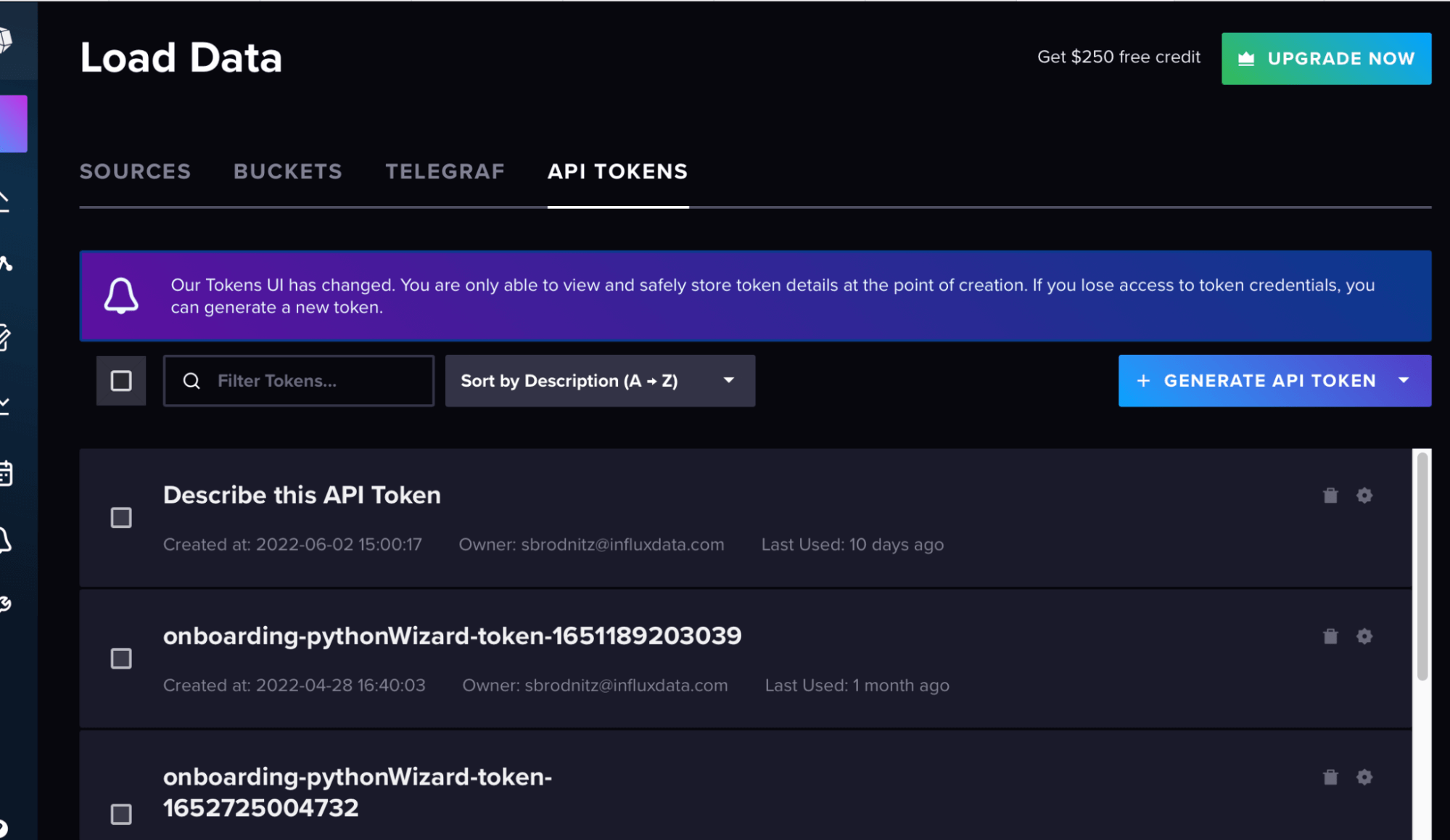
            points_to_send.append(p)

Then in the InfluxDB UI, create a bucket and token from the “load data” sidebar, as shown in these screenshots.

Your org is your email for the account, and the url is the url of your cloud account.

token=token
org = org
url = url
bucket = bucket

Here we set the batch size to 5,000 because that makes things more efficient, as described in the docs here.

with InfluxDBClient(url=url, token=token, org=org) as client:
    with client.write_api(write_options=WriteOptions(batch_size=5000)) as write_api:
        write_api.write(bucket=bucket, record=points_to_send)

Querying the data

Now that the data is in InfluxDB, we can query it. I’m going to use several queries to show you what each command does step by step. First, set up the query API.

client = influxdb_client.InfluxDBClient(url=url, token=token, org=org)
query_api = client.query_api()

Within your Jupyter notebook, each query is a string of Flux code, which you then call with the query API. In all of these cases, we have many options for what to do with the results of our queries. For the first ones, I’m going to print the first few results to make sure they’re working, and then finally we’ll end with a plot.

This query simply gathers all of the latitude, longitude and temperature fields.

query1='from(bucket: "sample_geo")\
  |> range(start: 2003-12-31, stop: 2020-01-01)\
  |> filter(fn: (r) => r["_measurement"] == "ocean_temperature")\
  |> filter(fn: (r) => r["_field"] == "lat" or r["_field"] == "temp" or r["_field"] == "lon")\
  |> yield(name: "all points")'

This query returns latitude.

query2='from(bucket: "sample_geo")\
  |> range(start: 2003-12-31, stop: 2020-01-01)\
  |> filter(fn: (r) => r["_measurement"] == "ocean_temperature")\
  |> filter(fn: (r) => r["_field"] == "lat")\
  |> yield(name: "lat")'

To execute either of these queries, and print the amount of points there are and the first few results, you can run the following, changing what query you’re passing in.

result = client.query_api().query(org=org, query=query2)
results = []
for table in result:
    for record in table.records:
        results.append((record.get_value(), record.get_field()))
print(len(results))
print(results[0:10])

Now we’re going to get started using the geo-temporal package. The geo.shapeData function reformats the data and assigns each point an S2 cell ID. You specify what your latitude and longitude field names are, “lat” and “lon” in this case, and what S2 cell level you want. In this case, I’ve chosen 10, which corresponds to an average of 1.27 kilometers squared. You can read about the cell levels here.

Next we’re going to use the geo.filterRows function to select the region we want to calculate the average temperature of. I’m picking a 150 kilometer circle centered around 20.5°N and 39.5°W, but you can pick any sort of box, circle or polygon as described here.

By default, the data is grouped by s2_cell_id, so to calculate a running mean over this whole region, we have to run the group function and tell it to group by nothing so all the data in the region is grouped together. Then you can use the aggregateWindow function to calculate running means and standard deviations over time windows of your choice.

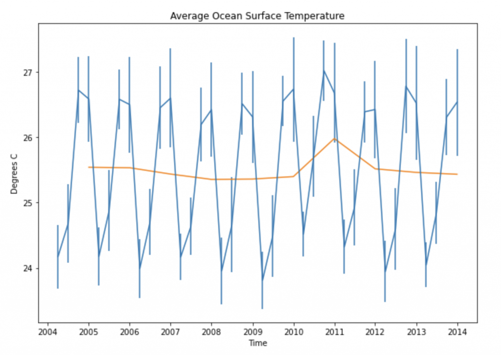
Putting this all together, the code below calculates and plots the mean over this circle every three months and every year, and the standard deviation every three months, which I’ve put as error bars in the plot below.

query3='import "experimental/geo"\
from(bucket: "sample_geo")\
    |> range(start: 2003-12-31, stop: 2020-01-01)\
    |> filter(fn: (r) => r["_measurement"] == "ocean_temperature")\
    |> geo.shapeData(latField: "lat", lonField: "lon", level: 13)\
    |> geo.filterRows(region: {lat: 20.5, lon: -39.5, radius: 150.0}, strict: true)\
    |> group()\
    |> aggregateWindow(column: "temp",every: 3mo, fn: mean, createEmpty: false)\
    |> yield(name: "running mean")\
    '

query4='import "experimental/geo"\
from(bucket: "sample_geo")\
    |> range(start: 2003-12-31, stop: 2020-01-01)\
    |> filter(fn: (r) => r["_measurement"] == "ocean_temperature")\
    |> geo.shapeData(latField: "lat", lonField: "lon", level: 13)\
    |> geo.filterRows(region: {lat: 20.5, lon: -39.5, radius: 150.0}, strict: true)\
    |> group()\
    |> aggregateWindow(column: "temp",every: 3mo, fn: stddev, createEmpty: false)\
    |> yield(name: "standard deviation")\
    '

query5='import "experimental/geo"\
from(bucket: "sample_geo")\
    |> range(start: 2003-12-31, stop: 2020-01-01)\
    |> filter(fn: (r) => r["_measurement"] == "ocean_temperature")\
    |> geo.shapeData(latField: "lat", lonField: "lon", level: 13)\
    |> geo.filterRows(region: {lat: 20.5, lon: -39.5, radius: 150.0}, strict: true)\
    |> group()\
    |> aggregateWindow(column: "temp",every: 12mo, fn: mean, createEmpty: false)\
    |> yield(name: "running mean")\
    '

result = client.query_api().query(org=org, query=query3)
results_mean = []
results_time = []
for table in result:
    for record in table.records:
        results_mean.append((record["temp"]))
        results_time.append((record["_time"]))

result = client.query_api().query(org=org, query=query4)
results_stddev = []
for table in result:
    for record in table.records:
        results_stddev.append((record["temp"]))
result = client.query_api().query(org=org, query=query5)

results_mean_annual = []
results_time_annual = []
for table in result:
    for record in table.records:
        results_mean_annual.append((record["temp"]))
        results_time_annual.append((record["_time"]))

plt.rcParams["figure.figsize"] = (10,7)
plt.errorbar(results_time,results_mean,results_stddev)
plt.plot(results_time_annual,results_mean_annual)
plt.xlabel("Time")
plt.ylabel("Degrees C")
plt.title("Average Ocean Surface Temperature")

Further resources

Using InfluxDB in Python makes geo-temporal analysis more efficient. I hope this example of the kinds of calculations you can do with this package sparks some ideas for you. This is really the tip of the iceberg. You can also use the package to calculate distances, find intersections, find whether certain regions contain specific points and more. And it can make an even bigger difference in saving computations with more complicated data sets with more points.

The combination of a platform built for time-series data and the S2 cell system is very powerful. For more information, you can read about the Flux geo-temporal package in our docs here and watch our Meet the Developers mini-series on the subject here.