Time Series Data Analysis
Definitions & Best Techniques for 2025
In this technical paper, InfluxData CTO, Paul Dix, will walk you through what time series is (and isn’t), what makes it different from stream processing, full-text search, and other solutions, and how to deliver real-time analytics.
Time series data and analysis
Time series analysis looks at data collected over time. For example, a time series metric could be the amount of inventory sold in a store from one day to the next. Often patterns emerge that can predict and prevent issues. A sudden drop in sales would be expensive for the company, so it would help to understand what events precede and predict this kind of change. Time series data is everywhere. As our world becomes increasingly instrumented, sensors and systems emit a relentless stream of time series data.
Examples of time series analysis:
- Electrical activity in the brain
- Rainfall measurements
- Stock prices
- Number of sunspots
- Annual retail sales
- Monthly subscribers
- Heartbeats per minute
Key time series concepts
- Time series data is a collection of data points over time.
- Time series analysis is identifying trends, like seasonality, to help forecast a future event.
Time series examples
Weather records, economic indicators and patient health evolution metrics—all are time series data. Time series data could also be server metrics, application performance monitoring, network data, sensor data, events, clicks and many other types of analytics data. The best way to understand time series is to start exploring with some sample data in InfluxDB Cloud.
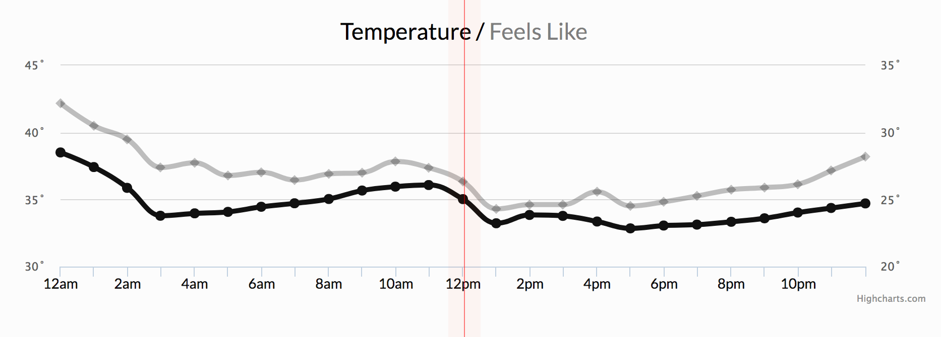
Notice how time—depicted at the bottom of the below chart—is the axis.
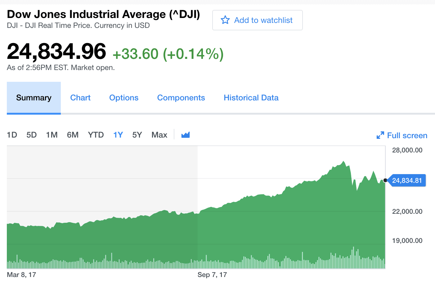
In the next chart below, note time as the axis over which stock price changes are measured. In investing, a time series tracks the movement of data points, such as a security’s price over a specified period of time with data points recorded at regular intervals. This can be tracked over the short term (such as a security’s price on the hour over the course of a business day) or the long term (such as a security’s price at close on the last day of every month over the course of five years).
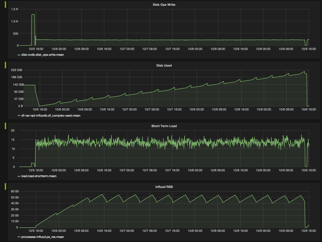
The cluster monitoring example below, depicting disk ops write and usage data, would be familiar to Network Operation Center teams. Remember that monitoring data is time series data.
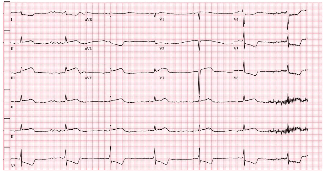
Another familiar example of time series data is patient health monitoring, such as in an electrocardiogram (ECG), which monitors the heart’s activity to show whether it is working normally.
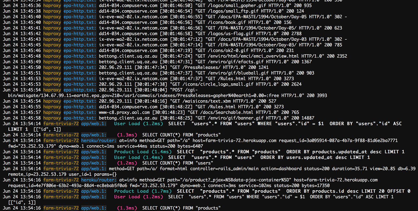
In addition to being captured at regular time intervals, time series data can be captured whenever it happens—regardless of the time interval, such as in logs. Logs are a registry of events, processes, messages and communication between software applications and the operating system. Every executable file produces a log file where all activities are noted. Log data is an important contextual source to triage and resolve issues. For example, in networking, an event log helps provide information about network traffic, usage and other conditions.
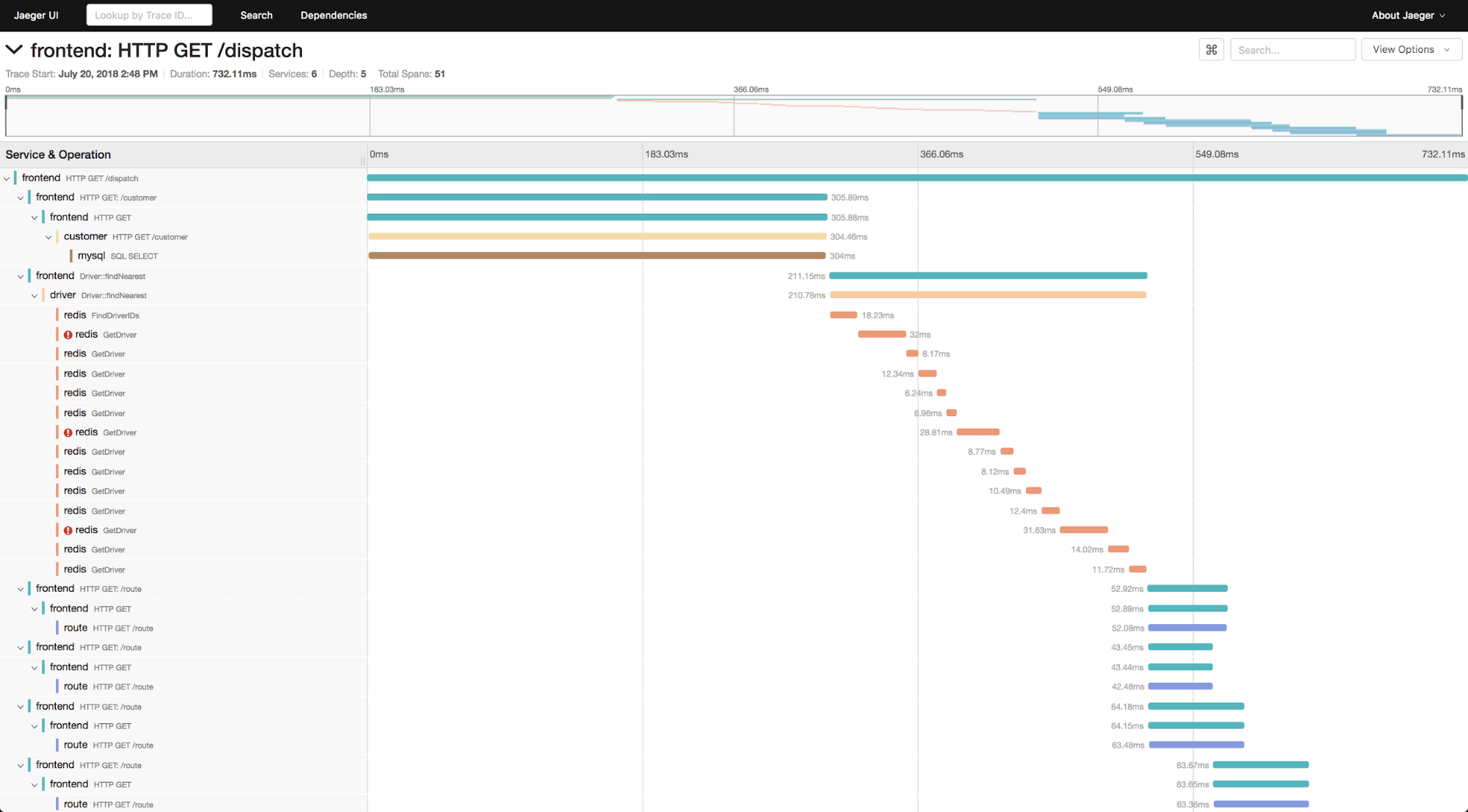
Traces (a list of the subroutine calls that an application performs during execution) are also time series data. Over the colored bands in the traces chart below, you can see examples of time series data. The goal of tracing is to follow a program’s flow and data progression. Tracing encompasses a wide, continuous view of an application to find bugs in a program or application.
The examples above encompass two different types of time series data, as explained below.
Types of time series data
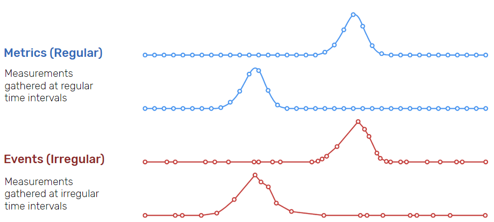
Time series data can be classified into two types:
- Measurements gathered at regular time intervals (metrics)
- Measurements gathered at irregular time intervals (events)
In the “Time series data examples” section above:
- Examples 3 (cluster monitoring) and 4 (health monitoring) depict metrics.
- Examples 5 (logs) and 6 (traces) depict events.
Because they happen at irregular intervals, events are unpredictable and cannot be modeled or forecasted since forecasting assumes that whatever happened in the past is a good indicator of what will happen in the future.
A time series data example can be any information sequence that was taken at specific time intervals (whether regular or irregular). Common data examples could be anything from heart rate to the unit price of store goods.
Linear vs. nonlinear time series data
A linear time series is one where, for each data point Xt, that data point can be viewed as a linear combination of past or future values or differences. Nonlinear time series are generated by nonlinear dynamic equations. They have features that cannot be modelled by linear processes: time-changing variance, asymmetric cycles, higher-moment structures, thresholds and breaks. Here are some important considerations when working with linear and nonlinear time series data:
- If a regression equation doesn’t follow the rules for a linear model, then it must be a nonlinear model.
- Nonlinear regression can fit an enormous variety of curves.
- The defining characteristic for both types of models are the functional forms.
Time series analysis
Analyzing time series data allows for extracting meaningful statistics and other data characteristics. As the name suggests, time series data is a collection of observations created by repeating measurements over time. Once you have that information, you can plot it on a graph and learn more about precisely what you’re tracking.
A very straightforward time series analysis example might be the rise and fall of the temperature over the course of a day. By tracking the specific temperature outside at hourly intervals for 24 hours, you have a complete picture of the rise and fall of the temperature in your area. Then, suppose you know that the next day will be relatively similar in terms of things like precipitation and humidity. In that case, you can make a more educated guess about the temperature at specific times. This analysis is an oversimplified example, yes—but the underlying structure is the same regardless of what it is that you’re talking about.
Such analysis requires identifying the pattern of an observed time series data set. Once the pattern is established, it can be interpreted, integrated with other data, and used for forecasting (fundamental for machine learning). Machine learning is a type of artificial intelligence that allows computer programs to actually “learn” and become “smarter” over time, all without being explicitly programmed to do so.
Importance of time series analysis
As more connected devices are implemented and data is expected to be collected and processed in real-time, the ability to handle time series data has become increasingly significant. This will become increasingly critical over the next few years as the Internet of Things, AI, and devices play an ever more important role in all of our lives.
At its core, the Internet of Things is a term used to describe a network of literally billions of connected devices — both creating and sharing data at all times. In a personal context, we’ve already seen this transition begin in “smart” homes across America. Your thermostat knows that when it gets to a certain temperature, it needs to lower the shades in a room to help control the temperature. Or your smart home hub knows that as soon as the last person leaves the house, it is to lock all the doors and turn all the lights off. It wouldn’t be able to get to this point were it not for an interconnected network of sensors exchanging information at all times—making time series analysis all the more critical.
Among other things, time series analysis can effectively - Illustrate that data points taken over time may have some sort of trend or pattern that likely otherwise would have gone undiscovered. - Provide users with a better understanding of the past, thus putting them in a position to better predict the future.
That last point is crucial and is a big part of why time series analysis is used in economics, statistics, and similar fields. Suppose you have historical data for a particular stock, for example, and you know how it has traditionally performed given certain world events. In that case, you can better predict the price when similar events occur in the future. If you know an economic downturn is coming, you can use that insight to make a better and more informed decision about purchasing the stock.
Since the analysis is based on data plotted against time, the first step is to plot the data and observe any patterns that might occur over time.
Want to learn more? Register for the Time Series Basics training or compare options for storing and analyzing time series data.
Time series analysis methods
Time series analysis is a method of analyzing a series of data points collected over a period of time. In time series analysis, data points are recorded at regular intervals over a set period of time, rather than intermittently or at random.
Time series analysis is the use of statistical methods to analyze time series data and extract meaningful statistics and characteristics about the data. TSA helps identify trends, cycles, and seasonal variances to aid in the forecasting of a future event. Factors relevant to TSA include stationarity, seasonality and autocorrelation.
Time series analysis can be useful to see how a given variable changes over time (while time itself, in time series data, is often the independent variable). Time series analysis can also be used to examine how the changes associated with the chosen data point compare to shifts in other variables over the same time period.
Time series forecasting methods
Time series forecasting uses information regarding historical values and associated patterns to predict future activity.
Time series forecasting methods include:
- Trend analysis
- Cyclical fluctuation analysis
- Seasonal pattern analysis
As with all forecasting methods, success is not guaranteed. Machine learning is often used for this purpose. So are its classical predecessors: Error, Trend, Seasonality Forecast (ETS), Autoregressive Integrated Moving Average (ARIMA) and Holt-Winters.
To ‘see things’ ahead of time, time series modeling (a forecasting method based on time series data) involves working on time-based data (years, days, hours, minutes) to derive hidden insights that inform decision-making. Time series models are very useful models when you have serially correlated data. Most businesses work on time series data to analyze sales projections for the next year, website traffic, competitive positioning and much more.
Learn more about time series forecasting methods, including decompositional models, smoothing-based models, and models including seasonality.
Identifying time series data
Time series data is unique in that it has a natural time order: the order in which the data was observed matters. The key difference with time series data from regular data is that you’re always asking questions about it over time. An often simple way to determine if the dataset you are working with is time series or not, is to see if one of your axes is time.
Time series considerations
Immutability – Since time series data comes in time order, it is almost always recorded in a new entry, and as such, should be immutable and append-only (appended to the existing data). It doesn’t usually change but is rather tacked on in the order that events happen. This property distinguishes time series data from relational data which is usually mutable and is stored in relational databases that do online transaction processing, where rows in databases are updated as the transactions are run and more or less randomly; taking an order for an existing customer, for instance, updates the customer table to add items purchased and also updates the inventory table to show that they are no longer available for sale.
The fact that time series data is ordered makes it unique in the data space because it often displays serial dependence. Serial dependence occurs when the value of a datapoint at one time is statistically dependent on another datapoint in another time (read “Autocorrelation in Time Series Data” for a detailed explanation about this topic).
Though there are no events that exist outside of time, there are events where time isn’t relevant. Time series data isn’t simply about things that happen in chronological order — it’s about events whose value increases when you add time as an axis. Time series data sometimes exists at high levels of granularity, as frequently as microseconds or even nanoseconds. With time series data, change over time is everything.
Different forms of time series data – Time series data is not always numeric — it can be int64, float64, bool, or string.
Time series data vs. cross-sectional and panel data
To determine whether your data is time series data, figure out what you’ll need to determine a unique record in the data set.
- If all you need is a timestamp, it’s probably time series data.
- If you need something other than a timestamp, it’s probably cross-sectional data.
- If you need a timestamp plus something else, like an ID, it’s probably panel data.
What the above means becomes clearer upon recalling the definition of (and differences between) each of these three data types:
Time series data definition
Time series data is a collection of observations (behavior) for a single subject (entity) at different time intervals (generally equally spaced as in the case of metrics, or unequally spaced as in the case of events).
For example: Max Temperature, Humidity and Wind (all three behaviors) in New York City (single entity) collected on First day of every year (multiple intervals of time)
The relevance of time as an axis makes time series data distinct from other types of data.
Cross-sectional data definition
Cross-sectional data is a collection of observations (behavior) for multiple subjects (entities such as different individuals or groups ) at a single point in time.
For example: Max Temperature, Humidity and Wind (all three behaviors) in New York City, SFO, Boston, Chicago (multiple entities) on 1/1/2015 (single instance)
In cross-sectional studies, there is no natural ordering of the observations (e.g. explaining people’s wages by reference to their respective education levels, where the individuals’ data could be entered in any order).
For example: the closing price of a group of 50 stocks at a given moment in time, an inventory of a given product in stock at a specific stores, and a list of grades obtained by a class of students on a given exam.
Panel data (longitudinal data) definition
Panel data is usually called as cross-sectional time series data as it is a combination of the above- mentioned types (i.e., collection of observations for multiple subjects at multiple instances).
Panel data or longitudinal data is multi-dimensional data involving measurements over time. Panel data contains observations of multiple phenomena obtained over multiple time periods for the same firms or individuals. A study that uses panel data is called a longitudinal study or panel study.
For example: Max Temperature, Humidity and Wind (all three behaviors) in New York City, SFO, Boston, Chicago (multiple entities) on the first day of every year (multiple intervals of time).
Differences between the three data types
Based on the above definitions and examples, let’s recap the differences between the three data types:
- A time series is a group of observations on a single entity over time — e.g. the daily closing prices over one year for a single financial security, or a single patient’s heart rate measured every minute over a one-hour procedure.
- A cross-section is a group of observations of multiple entities at a single time — e.g. today’s closing prices for each of the S&P 500 companies, or the heart rates of 100 patients at the beginning of the same procedure.
- If your data is organized in both dimensions — e.g. daily closing prices over one year for 500 companies — then you have panel data.
Time series analysis example using InfluxDB
To build a real-time risk monitoring system, Robinhood (a pioneer of commission-free investing) chose InfluxDB (a time series database built on open source technologies) and Faust (an open source Python stream processing library). The architecture behind their system involves both time series anomaly detection (InfluxDB) and real-time stream processing (Faust/Kafka).
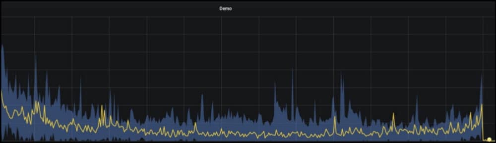
Robinhood alerted on the data with Faust, a real-time Python Library for Kafka Streams.
The aggregated data (yellow) is bounded by upper and lower limits (blue).
As the number of time series grows, the effort required to understand or detect anomalies in a time series becomes very costly. This is where an anomaly detection system can intelligently alert one when something doesn’t go very well.
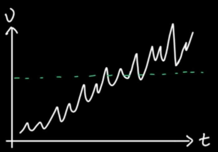
The first anomaly detection solution that Robinhood tried was threshold-based alerting, by which an alert is triggered whenever the underlying data is over or under the threshold. Threshold-based alerting works well with very simple time series but fails to account for more complex time series. As shown below, the time series here has a trend. It’s trending upwards, and there are some up-and-down patterns within that upward trend. If the fixed threshold is used to alert on anomalies, it doesn’t work well because it will go over the threshold, and will trigger an alert but will then drop down a threshold and go over a threshold again. So threshold-based alerting in the case of complex time series would require the same effort as checking the dashboard 24/7.
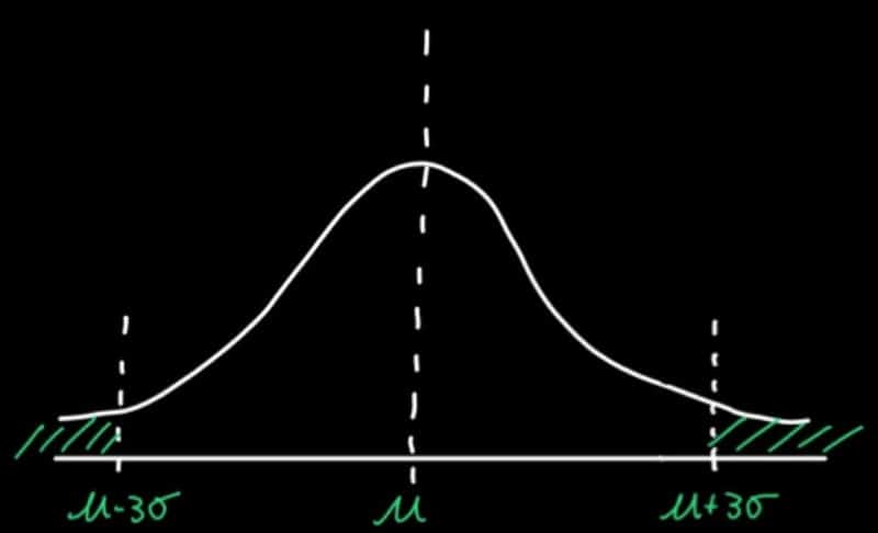
To fix this problem, Robinhood alerted on data outside of three standard deviations. Defining your threshold from a standard deviation for anomaly detection is advantageous because it can help you detect anomalies on data that is non-stationary (like the example above). In other words, the threshold defined by a standard deviation will follow your data’s trend. Robinhood defined an anomaly as anything outside of three standard deviations away from the mean — so 99.7% of the data lies within this range.
Applications in various domains
Time series models are used to:
- Gain an understanding of the underlying forces and structure that produced the observed data.
- Fit a model and proceed to forecasting, monitoring or feedback and feedforward control.
Applications span sectors such as:
- Budgetary analysis
- Census analysis
- Economic forecasting
- Inventory studies
- Process and quality control
- Sales forecasting
- Stock market analysis
- Utility studies
- Workload projections
- Yield projections
Understanding data stationarity
Stationarity is an important concept in time series analysis. Many useful analytical tools and statistical tests and models rely on stationarity to perform forecasting. For many cases involving time series, it’s sometimes necessary to determine if the data was generated by a stationary process, resulting in stationary time series data. Conversely, sometimes it’s useful to transform a non-stationary process into a stationary process in order to apply specific forecasting functions to it. A common method of stationarizing a time series is through a process called differencing, which can be used to remove any trend in the series which is not of interest.
Stationarity in a time series is defined by a constant mean, variance, and autocorrelation. While there are several ways in which a series can be non-stationary (for instance, an increasing variance over time), a series can only be stationary in one way (when all these properties do not change over time).
Patterns that may be present within time series data
The variation or movement in a series can be understood through the following three components: trend, seasonality, and residuals. The first two components represent systematic types of time series variability. The third represents statistical noise (analogous to the error terms included in various types of statistical models). To visually explore a series, time series are often formally partitioned into each of these three components through a procedure referred to as time series decomposition, in which a time series is decomposed into its constituent components.
Trend
Trend refers to any systematic change in the level of a series — i.e., its long-term direction. Both the direction and slope (rate of change) of a trend may remain constant or change throughout the course of the series.
Seasonality
Unlike the trend component, the seasonal component of a series is a repeating pattern of increase and decrease in the series that occurs consistently throughout its duration. Seasonality is commonly thought of as a cyclical or repeating pattern within a seasonal period of one year with seasonal or monthly seasons. However, seasons aren’t confined to that time scale — seasons can exist in the nanosecond range as well.
Residuals
Residuals constitute what’s left after you remove the seasonality and trend from the data.
Critical methods of analyzing time series data
Time series analysis methods may be divided into two classes:
- Frequency-domain methods (these include spectral analysis and wavelet analysis) In electronics, control systems engineering, and statistics, the frequency domain refers to the analysis of mathematical functions or signals with respect to frequency, rather than time.
- Time-domain methods (these include autocorrelation and cross-correlation analysis) Time domain refers to the analysis of mathematical functions, physical signals or time series of economic or environmental data, with respect to time. (In the time domain, correlation and analysis can be made in a filter-like manner using scaled correlation, thereby mitigating the need to operate in the frequency domain.)
Additionally, time series analysis methods may be divided into two other types:
- Parametric: The parametric approaches assume that the underlying stationary stochastic process has a certain structure which can be described using a small number of parameters (for example, using an autoregressive or moving average model). In these approaches, the task is to estimate the parameters of the model that describes the stochastic process.
- Non-parametric: By contrast, non-parametric approaches explicitly estimate the covariance or the spectrum of the process without assuming that the process has any particular structure.
Time series analysis best practices
For the best results in terms of time analysis, it’s important to gain a better understanding of exactly what you’re trying to do in the first place. Remember that in a time series, the independent variable is often time itself and you’re typically using it to try to predict what the future might hold.
To get to that point, you have to understand whether or not time is stationary, if there is seasonality, and if the variable is autocorrelated.
Autocorrelation is defined as the similarity of observations as a function of the amount of time that passes between them. Seasonality takes a look at specific, periodic fluctuations. If a time series is stationary, its own statistical properties do not change over time. To put it another way, the time series has a constant mean and variance regardless of what is happening with the independent variable of time itself. These are all questions that you should be answering prior to the performance of time series analysis.
Learn how Nobl9 Saved time and money with InfluxDB
Frequently asked questions (FAQ) about time series data
Where is time series data stored?
Time series data is often ingested in massive volumes and requires a purpose-built database designed to handle its scale. Properties that make time series data very different than other data workloads are data lifecycle management, summarization, and large range scans of many records. This is why time series data is best stored in a time series database built specifically for handling metrics and events or measurements that are time-stamped.
Learn more about time series data storage and about the best way to store, collect and analyze time series data.
What is a time series statistic?
A time series statistic refers to the data extracted from a time series model. The information must be recorded over regular time intervals, and may be combined with cross-sectional data to derive relevant predictions.
What are time plot statistics?
Time plot statistics refer to the evolution of a series over a specific time interval. It’s often used at the beginning of an analysis for quick interpretation of anything from trends to anomalies.
Is a time series database the same as a data warehouse or data lakehouse?
No, but the data warehousing process helps you analyze data that exists in all the systems and software tools in your organization, including a time series database. Read more on how InfluxDB works with your data lakehouse.
How is time series data understood and used?
Time series data is gathered, stored, visualized and analyzed for various purposes across various domains:
- In data mining, pattern recognition and machine learning, time series analysis is used for clustering, classification, query by content, anomaly detection and forecasting.
- In signal processing, control engineering and communication engineering, time series data is used for signal detection and estimation.
- In statistics, econometrics, quantitative finance, seismology, meteorology, and geophysics the time series analysis is used for forecasting.
What is a time series graph?
Time series graphs are simply plots of time series data on one axis (typically Y) against time on the other axis (typically X). Graphs of time series data points can often illustrate trends or patterns in a more accessible, intuitive way.

