Community Highlight: How Supralog Built an Online Incremental Machine Learning Pipeline with InfluxDB OSS for Capacity Planning
By
Community
Product
Use Cases
Developer
Jul 02, 2020
Navigate to:
This article was written by Gregory Scafarto, Data Scientist intern at Supralog, in collaboration with InfluxData’s DevRel Anais Dotis-Georgiou.
At InfluxData, we pride ourselves on our awesome InfluxDB Community. We’re grateful for all of your contributions and feedback. Whether it’s Telegraf plugins, community templates, awesome InfluxDB projects, or Third Party Flux Packages, your contributions continue to both impress and humble us. Today, let’s shine a spotlight on Gregory Scafarto from Supralog.
Gregory Scafarto built and maintains an online capacity planning pipeline with Kapacitor, Python, and InfluxDB. Gregory Scafarto is based in France and is finishing the last year of his Masters Degree in Computer Systems Networking and Telecommunication at ENSEIRB-MATMECA. He’s also working as a Data Scientist intern at Supralog on research for predictive maintenance and capacity planning solutions.
How Supralog uses Kapacitor for capacity planning
Capacity planning is one of the most important types of analysis in time series monitoring. Capacity planning tools help evaluate the production capacity required by an organization. Specifically in IT, capacity planning involves estimating the storage, business demand, and cost estimates to deliver the agreed service level targets.
The setup:
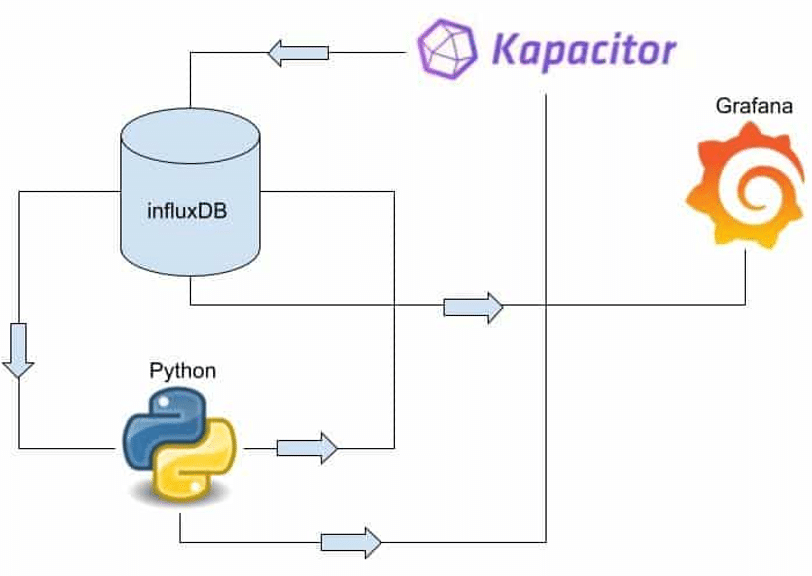
Supralog decided to use InfluxDB’s TICK Stack for many reasons. It’s highly performant and easy to use, but one stack element stood out: Kapacitor, an alerting and real-time stream data processing engine that works with Python and handles our time series forecasting. We use Kapacitor and InfluxDB to perform online machine learning to generate a large amount of CPU, memory, and disk usage predictions. We plan to extend this architecture to generate predictions on website traffic, email traffic, and other application performance metrics.
We write and query data with the InfluxDB-Python Client and use Python for data preparation and forecasting. Our Python script also calculates the residuals, the difference between the prediction and the real value. Kapacitor alerts on those prediction residuals to apply continuing learning to our machine learning (ML) model. If the prediction residuals are too large and the model accuracy is drifting, the model is retrained on a new training set of data to optimize the model for accuracy. Grafana is only used for visualization purposes.
Note: In an attempt to limit this blog to key components of the architecture above, this tutorial will not cover all of the code in detail. Please take a look at Gregory’s accompanying repo here.
Disadvantages of FB Prophet for capacity planning at scale
Our prediction architecture evolved over time. At first, the predictions were made with Facebook Prophet, a “forecasting procedure implemented in R and Python”, which has a high-level API and allows users to make predictions very quickly. However, we ended up removing Prophet from our pipeline because it presents some disadvantages for our use case:
- It has a tendency to smooth curves.
- It doesn't have "online training". Instead, the model must be trained on a complete cycle of data each time the model drifts. This disadvantage is very expensive because it requires a lot of CPU and RAM resources, especially given the hundred predictions we're making.
Data preparation and data validation
Data preparation is the process of transforming raw data into a form that is valuable for subsequent analysis or machine learning applications. Data validation is the process of ensuring that our data has undergone the proper data preparation.
Step One: Data preparation
The first step is to extract the data from the database with the InfluxDB-Python Client and transform it into a Pandas DataFrame. Next, we perform some time series data analytics to group our data into two seperate groups to determine which prediction methods should be applied to the data. Specifically, we use time series decomposition to group our data. We chose to separate our time series into two distinct groups:
- Group One: data with trend, but without seasonality. Group One data predictions are made with a classical model. Specifically, Group One data predictions are made with linear regression.
- Group Two: data with trend and seasonality. Group Two data predictions are made which will employ a machine learning model. Specifically, Group Two data predictions are made with a Long short-term memory Network (LSTM).
In this first example, this time series represents percentage of disk usage from host:
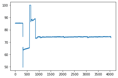
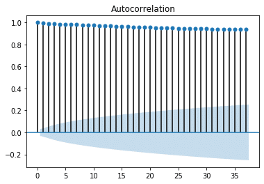
We can easily see that the data seems to be piecewise linear it is composed of straight-line segments but we need to determine which group it belongs to. We wrote a test that can automatically detect the nature of the time series. This test first computes the autocorrelation function. Autocorrelation is a measure of the correlation of a time series with itself at a previous point in time. Autocorrelation plots can help us to determine whether or not a time series has seasonality. To learn more about autocorrelation, what it tells us, and its effect on ML models, take a look at this blog. Plotting the autocorrelation of the data above gives us a signal like this:
Step Two: Data validation
Through visual inspection, the plot verifies that our data doesn’t exhibit seasonality, which places it in Group One. However, we need a quantifiable way to reach this conclusion so we can determine whether data has seasonality automatically. We take the Pearson’s Correlation Coefficient (R) of the autocorrelation function in order to automate the grouping of our time series data and determine if our time series is going to be well-modeled by a linear model or a ML model. The Pearson’s correlation coefficient is the measure of magnitude of linear correlation between two variables. It is defined by this mathematical formula:

where,

An R=±1 indicates strong linear correlation where a R=0 indicates no linear correlation.
A linear regression forecasting model with InfluxDB and Python
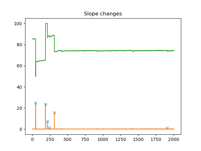
Now that we’ve determined that our data will require a linear prediction model, we must decide what data to feed into our model. We can’t use all the data to make the linear model as the slope changes with time. Using all the data would obscure recent and relevant changes in slope. One solution to this problem is to determine the last meaningful slope change and only select the portion of the time series that contains the most recent significant change. This ensures that our forecast will be made based on the most relevant and meaningful trend.
In order to find those useful slope changes we will take the absolute derivative of the series and then find the significant derivative peaks. We define significant derivative peaks by a simple threshold, which is used in signal.find_peaks function from SciPy, as seen in the code below. To decrease signal noise and ensure that only relatively significant peaks are selected, a while loop is used to limit the number of peaks returned to the top 10% largest peaks. At each loop we increase the height of the peak threshold by one percent in order to drop noisy, smaller peaks. We iterate until we have the top 10% of peaks.
Here is an example of the results of such operations in our signal:
Here’s the code for the training of our linear model, Make_Linear_Model.py, complete with the while loop for eliminating smaller relatively insignificant peaks. Once we have analyzed the derivative peaks, we then apply linear regression to our time series at the presence of those peaks and generate a linear forecast.
import numpy as np
import matplotlib.pyplot as plt
from sklearn.linear_model import LinearRegression
from numpy import diff
from scipy.signal import find_peaks

def train_linear_model(df,severity):
    '''
    Determine the last linear part of data to consider and then train the model of this subsequence of data.

    Parameters
    ----------
    df : dataframe
        data.
    severity : int
       how insensitive will the model be to small changes

    Returns
    -------
    model : linear_model
        linear model trained on the last trend of the signal.
    r_sq : int
        Pearson's coefficient (caracterize how well the model represent the data).
    df_l : dataframe
        last linear part of the data.

    '''
    dx = 1
    dy = diff(df["y"])/dx
    i=1
    mini=np.amin(df["y"])
    maxi=np.amax(df["y"])
    j=0
    nb_peaks = len(df["y"])+1
    while nb_peaks > len(df["y"])/10 :
        peaks, _ = find_peaks(abs(dy), height=(severity+j)*(maxi-mini)/100)
        nb_peaks=len(peaks)
        j=j+1
        plt.plot(peaks, abs(dy[peaks]), "x")
        plt.plot(abs(dy))
        plt.plot(df["y"])
        plt.title("Slope changes")
        plt.show()
    i=peaks[-1]+1
    df_l=df["y"][i+1 :]
    x=np.linspace(1,len(df_l)-1,len(df_l))
    model = LinearRegression()
    model.fit(x.reshape(-1,1),np.asarray(df_l).reshape(-1,1))
    r_sq=model.score(x.reshape(-1,1), np.asarray(df_l).reshape(-1,1))
    return model,r_sq,df_l
Data preparation for our machine learning forecasting model with InfluxDB and Python
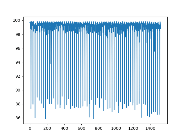
Now let’s focus on Group Two, non-linear data with seasonality, that employs machine learning for its prediction. Group Two contains available CPU percent data from a variety of hosts. Here is what our raw data looks like for one host:
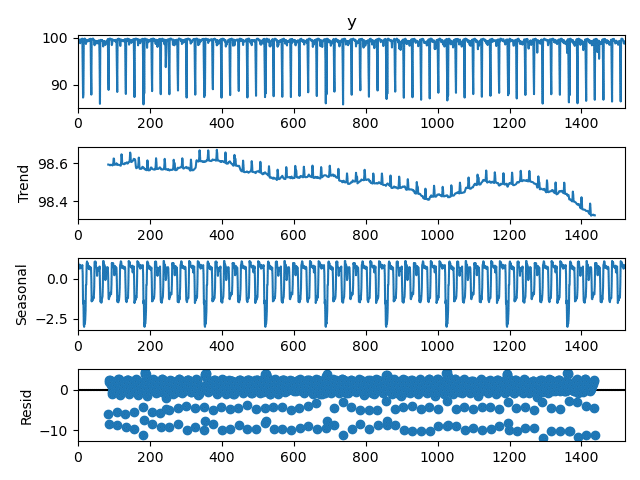
First, we perform time series decomposition and separate our series into three time series components: trend, seasonality and residual or “noise”. We perform decomposition because we process each component in a separate LSTM network. We use the seasonal_decompose function from Statsmodels, a “Python module that provides classes and functions for the estimation of many different statistical models”, to perform the decomposition. This Statsmodels seasonal decomposition function requires that the user specify a period. We selected a period of 24*7 +1 (a week if the data is sampled at 1-hour frequency) as the data has weekly seasonal periods. It is really important to make sure that your seasonal period is accurate. If you use an incorrect period, then the decomposition is poor and our model becomes inaccurate. This is also why verifying the presence and seasonal period with autocorrelation plots is so important.
We also used the additive method of the Statsmodels seasonal decomposition function to make reconstruction of the final time series easy. Since we select an additive method for our decomposition, our final prediction is made by adding the individual component predictions together to regenerate the time series. By using the decomposition method, we lose 12 points because of the edge effect due to the filter used by the Statsmodels seasonal decomposition function (which uses a moving average filter of size 13). Therefore, the predicted points are shifted back by 12 time steps in the past in order to be time accurate.
LSTMs briefly explained
Before we dive into how we used Keras, a ML framework, and LSTMs for incremental learning, let’s take a moment to briefly introduce LSTMs. This section will only skim the surface of LSTMs. If you’re interested in learning about LSTMs in depth, this blog provides an excellent explanation of how LSTMs work.
We use three LSTMs to output predictions for each of our decomposed components of our time series. We use LSTMs (Long Short Term Memory) Networks to model our seasonal time series because they specialize in learning dependencies in time series patterns over long periods. The following internal properties make LSTMs a very powerful time series model:
- LSTMs accept data sequences as inputs. A data sequence can just be a single array of values. This reduces the amount of data preparation required in order to use LSTMs.
- LSTM data processing is bidirectional and it has a memory state, which helps avoid the gradient vanishing problem, a common deep neural networks problem. In other words, LSTMs are good at training quickly.
The following diagram represents a LSTM cell and summarizes the networks function:

A LSTM network cell is composed of three main components or gates:
- An input gate decides which values and components of our time series get updated as they pass through the cell.
- A forget gate determines which values are forgotten or persist in the "memory" of the network. This forget gate makes LSTMs good at retaining learning time series patterns over long periods. This is a characteristic part of LSTMs.
- An output gate which determines the information to be passed to the next cell and ultimately outputs a prediction.
Using Keras for time series predictions for InfluxDB
Now we’re ready to take a look at the code which makes predictions on our three time series components. We used Keras, an open source neural network library that is a wrapper for TensorFlow to apply LSTMs. We decided to use Keras because it easily enables incremental learning. Incremental learning is a machine learning technique where new data is continuously fed into the model to further train the model and increase model accuracy efficiently. For example, we only need to query a week of data from our InfluxDB instance to retrain our model. Incremental learning is more efficient, resource-conscious, and cheaper than the traditional machine learning approach which requires querying all our historical data to retrain our model. Here is our Making_ML_Model.py code which implements an incremental learning LSTM network with Keras:
from keras.models import Sequential,save_model
from keras.layers import Dense,LSTM,Dropout

def make_models(nb_layers,loss,,nb_features,optimizer,look_back) :
    '''
    Create an LSTM model depending on the parameters selected by the user

    Parameters
    ----------
    nb_layers : int
        nb of layers of the lstm model.
    loss : str
        loss of the model.
    metric : str
        metric to evaluate the model.
    nb_features : int
        size of the ouput (one for regression).
    optimizer : str
        gradient descend's optimizer.
   look_back : int
       windows to be process by the network to make the prediction
    trend : bool
          Distinguish trend signal from others (more complicated to modelise).

    Returns
    -------
    model : Sequential object
        model
    '''
    model=Sequential()
    model.add(LSTM(nb_layers,return_sequences=True,activation='relu',input_shape=(nb_features,.look_back)))
    model.add(Dropout(0.2))
    model.add(LSTM(nb_layers))
    model.add(Dropout(0.2))
    model.add(Dense(int(nb_layers/2),activation='relu'))
    model.add(Dense(1))
    model.compile(loss=loss,optimizer=optimizer,metrics=["mse"])
    print("model_made")
    return model
To learn more about how this code works and to use an LSTM to generate a univariate time series prediction, I recommend checking out this blog.
Evaluating our machine learning model
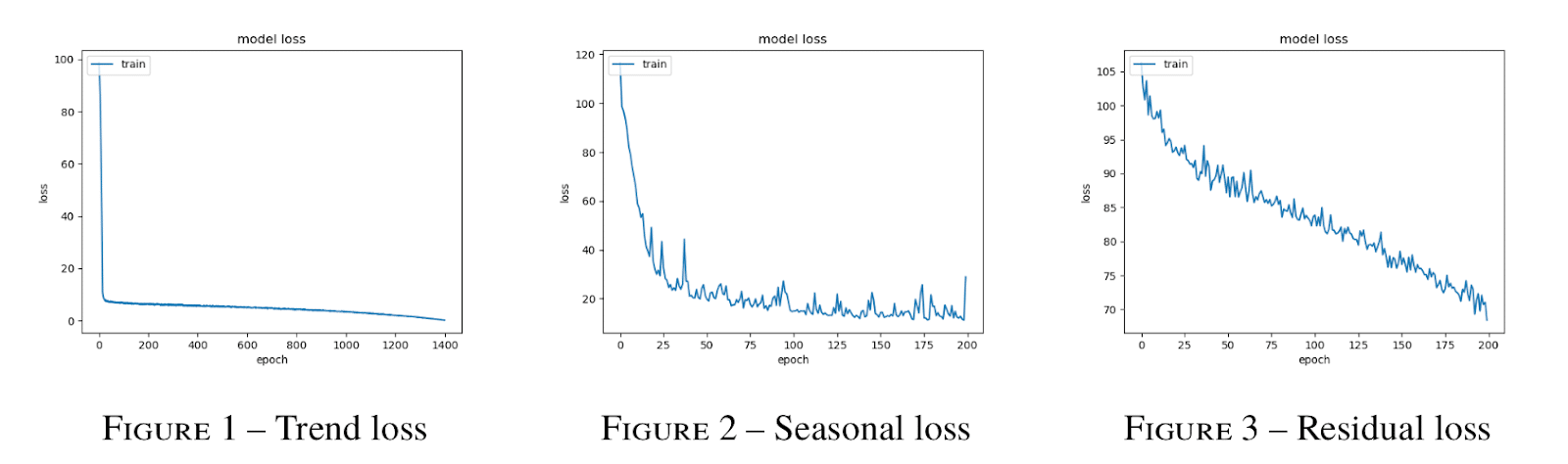
It’s always valuable to plot the losses of our models to evaluate whether training was successful. We can look at our model’s training loss for our three components: trend, seasonality, and residuals. Training loss is a measure of the penalty for a bad prediction during training. The higher the loss, the worse the prediction is.
- Generally, training loss decreases as you increase the number of training epochs, or one pass of the complete dataset through the model.
- At each epoch, the network computes the loss function value and updates the gradient in order to minimize the loss function.
In other words, the more times the model gets to consume the dataset, the more opportunities the model has to improve.
When the training loss reaches a saturation minimum, or stops decreasing, the model has “learned all that it can” and is accurate as it can be. From the graphs above, we see that we could make more epochs in order to improve the accuracy of prediction as the losses look like they haven’t finished decreasing. However, increasing the epochs increases the duration of the training. We need to strike a compromise between accuracy improvement and training duration.
Residuals help determine model confidence intervals
Time series residuals or noise tend to contribute the largest uncertainty to the model because of the very nature of seasonal decomposition and residuals themselves. However, since the residuals typically have a Gaussian distribution, we can easily compute a 95% confidence interval with the following formula:
![]()
Calculating the prediction intervals for the noise provides us with a good way to measure the minimum uncertainty of the entire model since it contributes the most error. However, it’s worth noting that measuring uncertainty through this approach is only effective for short predictions, but loses accuracy for longer predictions. This approach is used because it provides a good approximation of the uncertainty and is more computationally efficient than the methodology for calculating the true uncertainty of the final model as described in Deep and Confident Prediction for Time Series at Uber.
Our composite LSTM's predictions, the addition of the individual predictions
After predictions are made for trend, seasonality and residuals, those predictions are added together. Here are the results of our prediction one week into the future complete with confidence intervals:
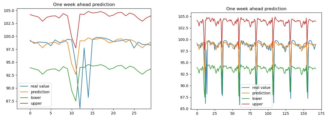
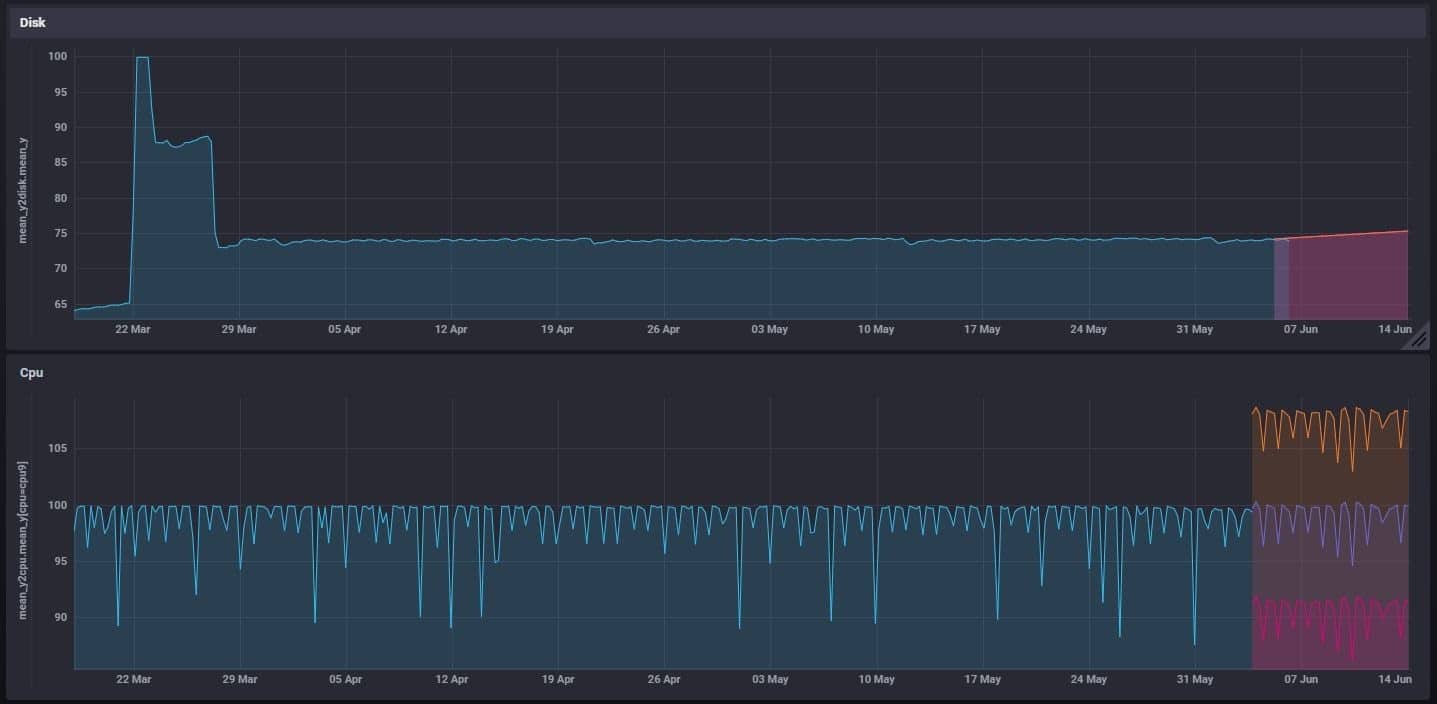
The plot on the left is zoomed in on a portion of our prediction so we can better visualize how well our prediction fits our real value it looks pretty good! Finally, now that we have a prediction, we write it to our InfluxDB instance with the client. Here is the output on our Grafana dashboard:
Alerting on residuals with Kapacitor and performing incremental learning with the exec() node
We’re almost at the end! All that’s left to do is to:
- Create Kapacitor's alert to monitor the error of residuals
- Create the online incremental training method script that executes our retraining script properly
We use Kapacitor to perform math across measurements and trigger alerts. Specifically, we’ll use Kapacitor to monitor our prediction residuals and relaunch training if the model drifts. Kapacitor is able to do a lot, but today we’ll focus on the exec() node which is able to launch scripts if the conditions of our alert are met. This is the heart of our TICK script. Here is our TICK script:
import os

path_to_kap = os.environ['kapacitor']
path_to_script = os.environ['script']

class Alert():
    def __init__(self,host,measurement) :
        self.host=host
        self.measurement=measurement
        self.texte=""

    def create(self,message,form):
        self.form=form
        '''
        Create the tick alert
        Note : NEED TO DEFINE the path of the script, which will be launched when an alert is triggered, as a variable environnement

        Parameters
        ----------
        message : str
            Message to be shown as an alert on slack etc ; need to be written with kapacitor syntax
        form : str
            ex ,host=GSCA,device=device1  group by conditions with comma to separate + start with a comma

        Returns
        -------
        None.

        '''
        where_condition=""
        where=[[element.split("=") for element in form[1 :].split(",")][i][0]for i in range(len(form[1 :].split(",")))]
        for ele in where :
            where_condition=where_condition+ele+"="+ele +" AND "
        texte=""
        cond=["var "+(form[1 :].replace(","," AND").split("AND")[i]).replace("=","='")+"'" for i in range(len(form[1 :].replace(","," AND").split("AND")))]
        for element in cond :
            texte=texte+element+"\n"
        texte = texte +"\n\n"+ """var realtime = batch
                |query('SELECT mean(yhat) as real_value FROM "telegraf"."autogen".real_"""+self.measurement+""" WHERE """+where_condition[: -5]+"""')
                    .period(6h)
                    .every(6h)
                    .align()
                |last('real_value')
                    .as('real_value')

            var predicted = batch
                |query('SELECT mean(yhat) as prediction FROM "telegraf"."autogen".pred_"""+self.measurement+""" WHERE """+where_condition[: -5]+"""')
                    .period(6h)
                    .every(6h)
                    .align()
                |last('prediction')
                    .as('prediction')

            var joined_data = realtime
                |join(predicted)
                    .as('realtime', 'predicted')
                    .tolerance(20m)

            var performance_error = joined_data
                |eval(lambda: abs("realtime.real_value" - "predicted.prediction"))
                    .as('performance_error')
                |alert()
                    .crit(lambda: "performance_error" > 10 )
                    .message('""" +message+"""')
                    .slack()
                    .exec('"""+path_to_script+"""', '"""+self.host+"'"+""", '"""+str(form[1 :])+"'"+""")

        self.texte=texte
    def save_alert(self):
        self.form=self.form[1 :].replace("=",".")
        self.form=self.form.replace(",","_")
        self.form=self.form.replace(":","")
        self.path=r"Alertes/alerte_"+self.host+"_"+self.form+".tick"   #path to modifie as you want
        with open(self.path,"w") as f :
            f.write(self.texte)
        f.close()

    def define_alert(self):
        self.form=self.form.replace("=",".")
        self.form=self.form.replace(",","_")
        self.form=self.form.replace(":","")
        cmd_define_alert=path_to_kap+" define "+"alerte_"+self.host+"_"+self.form+" -type batch -tick "+self.path+" -dbrp telegraf.autogen"
        print(cmd_define_alert)
        os.system('cmd /c '+cmd_define_alert)

    def enable_alert(self):
        self.form=self.form.replace("=",".")
        self.form=self.form.replace(",","_")
        self.form=self.form.replace(":","")
        cmd_enable_alert=path_to_kap+" enable "+"alerte_"+self.host+"_"+self.form
        os.system('cmd /c '+cmd_enable_alert)

    def launch(self):
        self.define_alert()
        self.enable_alert()
The Alert() class creates an alert adapted with the model we’ve created in order to monitor our prediction and relaunch a training if the model drifts. The create() function joins our prediction measurement with our actual data, calculates the prediction residual or model drift, sends an alert to Slack when a retraining event occurs, and runs our intermediate script with the exec() node. Please note that the path to Kapacitor and the intermediate scripts are written as environment variables because in our case the script will be put in production on a Docker’s container.
Now let’s explain what the intermediate script does, but first, remember our Python Keras script needs to import non-trivial modules and libraries. At the start of the project, a virtual environment was created at the root of the project directory with: python -m venv name_venv. Our intermediate script activates this virtual environment which contains several packages (including pip) and directories (including Script which contains activate.bat). The intermediate script contains one line:
For Windows:
%activate_project% && cd %ml_project_directory% && python Retrain.py %1 %2 %3where %activate_project% is the path to \Scripts\activate.bat from the venv directory
and %ml_project_directory% the path to the root of your project containing the Retrain.py directory added to your path variables.
For Linux or MacOS:
%activate_project && cd %ml_project_directory && python Retrain.py %1 %2 %3where %activate_project is the path to \Scripts\bin\activate.bat from the venv directory and %ml_project_directory the path to the root of your project containing the Retrain.py directory added to your path variables.
The intermediate script is a .bat that activates the virtual environment and then runs the retraining python code,Retrain.py. The Retrain.py reuses functions from the first training file but the models pick up from where they left off. They do so by applying the latest HDF5 files, which store the weights of each model (i.e. trend.h5, seasonality.h5, and residuals.h5), for each forecasted series during retraining. These files are stored in the forecasted series’ corresponding directory. For example, assume we are forecasting CPU. Then in the script above:
%1a string that represents the host of interesthost1%2a string that represents the measurementcpu%3a string that represents the series key in line protocolhost=host1,cpu=cpu-total. It represents the form in theExisting_Predictor()class in the script below.
For each series, the corresponding directory has the following name: primaryTag_measurement_seriesKey. For the example above, our model’s weights directory for that series would be host1_cpu_host1_cpu-total.
Here is the script that contains the load_models() function. The load_modules() function splits the form, %3, and specifies the directory from where the weights will be loaded from.
class Existing_Predictor(Predictor):

    def __init__(self,df,host,measurement,look_back,nb_epochs,nb_batch,form,freq_period) :
        Predictor.__init__(self)
        self.df=df
        self.host=host
        self.measurement=measurement
        self.form=form
        self.look_back=look_back
        trend_x, trend_y,seasonal_x,seasonal_y,residual_x,residual_y=self.prepare_data(df,look_back,freq_period)
        model_trend,model_seasonal,model_residual=self.load_models()
        model_trend=self.train_model(model_trend,trend_x,trend_y,nb_epochs,nb_batch,"trend")
        model_seasonal=self.train_model(model_seasonal,seasonal_x,seasonal_y,nb_epochs,nb_batch,"seasonal")
        model_residual=self.train_model(model_residual,residual_x,residual_y,nb_epochs,nb_batch,"residual")
        self.model_trend=model_trend
        self.model_seasonal=model_seasonal
        self.model_residual=model_residual

    def load_models(self):
        file=""
        for element in self.form :
            value=element.split("=")
            file=file+'_'+value[1]
        file=file[1 :].replace(":","")
        model_trend=load_model("Modeles/"+file+"_"+self.measurement+"/"+"trend"+".h5")
        model_seasonal=load_model("Modeles/"+file+"_"+self.measurement+"/"+"seasonal"+".h5")
        model_residual=load_model("Modeles/"+file+"_"+self.measurement+"/"+"residual"+".h5")
        return model_trend,model_seasonal,model_residual
At this point the intermediate script has run and in turn successfully retrained our model. Congrats, you have created an autonomous module doing predictions depending on the nature of the metric and frame it with an 95% confidence interval.
As mentioned previously, only a portion of the code used in this project is shared in this blog. Please take a look at this repo to learn about the prepare_data(), train_model() and save_model() methods that complete this ML approach.
Online machine learning with InfluxDB 2 and final thoughts from InfluxData
The following section is a note from Anais Dotis-Georgiou, DevRel at InfluxData.
It’s apparent that Gregory is a Data Science ninja, and I am grateful for him sharing his story. However, if you look at his code and his approach, you know he’s using InfluxDB 1.x and Kapacitor. Gregory started on his journey with the 1.x TICK Stack. Those of you getting started now might ask, “How can I accomplish this with InfluxDB 2.0?” Here is how you can create a similar forecasting pipeline with InfluxDB 2.0:
- Use the new Python Client. This allows you to query and write pandas DataFrames directly. It's also compatible with 1.x in case you feel uncomfortable using 2.0 which is currently in beta. (We recently announced at InfluxDays that we intend to make InfluxDB 2.0 OSS generally available in the fall, while InfluxDB Cloud is generally available now!).
- Calculate the prediction residuals with Flux and joins. I would also calculate Pearson's Correlation Coefficient with the pearsonr() function.
- Write the residuals to a new bucket or measurement with the to() function. I would execute this Flux Script on a regular interval with a Task.
- Use Alerts and the http.post() function to trigger retraining and run scripts. Alternatively, you could also consider using Node-RED, a "programming tool for wiring together hardware devices", to trigger retraining.You might also be interested in reading this blog that bears some similarity with that proposed architecture approach. It describes how Node-RED is used for continuous deployment of Telegraf Configurations.
Regardless of which edition or version of InfluxDB you are using, I hope this story inspires you to integrate machine learning into your InfluxDB-powered solution. Again, I’d like to thank Gregory for sharing his story and thank the InfluxData community for all of your contributions. As always, please share your thoughts, concerns, or questions in the comments section, on our community site, or in our Slack channel. We’d love to get your feedback and help you with any problems you run into!
Also, since this article’s topic interests you, watch the No-Code ML for Forecasting and Anomaly Detection webinar. It describes a POC for a containerized, no-code approach to ML with InfluxDB. You can also share your thoughts with the presenter Dean Sheehan.
