How We Did It: Data Ingest and Compression Gains in InfluxDB 3.0

By Rick Spencer / Product, Company
Oct 04, 2023

A few weeks ago, we published some benchmarking that showed performance gains in InfluxDB 3.0 that are orders of magnitude better than previous versions of InfluxDB – and by extension, other databases as well. There are two key factors that influence these gains: 1. Data ingest, and 2. Data compression. This begs the question, just how did we achieve such drastic improvements in our core database?

This post sets out to explain how we accomplished these improvements for anyone interested.

A review of TSM

To understand where we ended up, it’s important to understand where we came from. The storage engine that powered InfluxDB 1.x and 2.x was something we called the InfluxDB Time-Structured Merge Tree (TSM). Let’s take a brief look at data ingest and compression in TSM.

TSM data model

There’s a lot of information out there about the TSM data model, but if you want a quick overview, check out the information in the TSM docs here. Using that as a primer, let’s turn our attention to data ingest.

TSM ingest

TSM uses an inverted index to map metadata to a specific series on disk. If a write operation adds a new measurement or tag key/value pair, then TSM updates the inverted index. TSM needs to write this data in the proper place on disk, essentially indexing it when written. This whole process requires a significant amount of CPU and RAM.

The TSM engine sharded files by time, which allowed the database to enforce retention policies, evicting expired data.

Introduction of TSI

Prior to 2017, InfluxDB calculated the inverted index on startup, maintained it during writes, and kept it in memory. This led to very long startup times, so in the autumn of 2017, we introduced the Time Series Index (TSI), which is essentially the inverted index persisted to disk. This created another challenge, however, because the size of TSI on disk could become very large, especially for high cardinality use cases.

TSM compression

TSM uses run length encoding for compression. This approach is very efficient for metrics use cases where data timestamps occurred at regular intervals. InfluxDB was able to store the starting time and time interval, and then calculate each time stamp at query time, based on only row count. Additionally, the TSM engine could use run length encoding on the actual field data. So, in cases where data did not change frequently and the timestamps were regular, InfluxDB could compress data very efficiently.

However, use cases with irregular timestamp intervals, or where the data changed with nearly every reading, reduced the effectiveness of compression. The TSI complicated matters further because it could get very large in high cardinality use cases. This meant that InfluxDB hit practical compression limits.

Introduction of InfluxDB 3.0

When we embarked upon architecting InfluxDB 3.0, we were determined to solve these limitations related to ingest efficiency and compression, and to remove cardinality limitations to make InfluxDB effective for a wider range time series use cases.

3.0 Data model

We started by rethinking the data model from the ground up. While we retain the notion of separating data into databases, rather than persisting time series, InfluxDB 3.0 persists data by table. In the 3.0 world, a “table” is analogous to a “measurement” in InfluxDB 1.x and 2.x.

InfluxDB 3.0 shards each table on disk by day and persists that data in the Parquet file format. Visualizing that data on disk looks like a set of Parquet files. The database’s default behavior generates a new Parquet file every fifteen minutes. Later, the compaction process can take those files and coalesce them into larger files where each file represents one day of data for a single measurement. The caveat here is that we limit the size of each Parquet file to 100 megabytes, so heavy users may have multiple files per day.

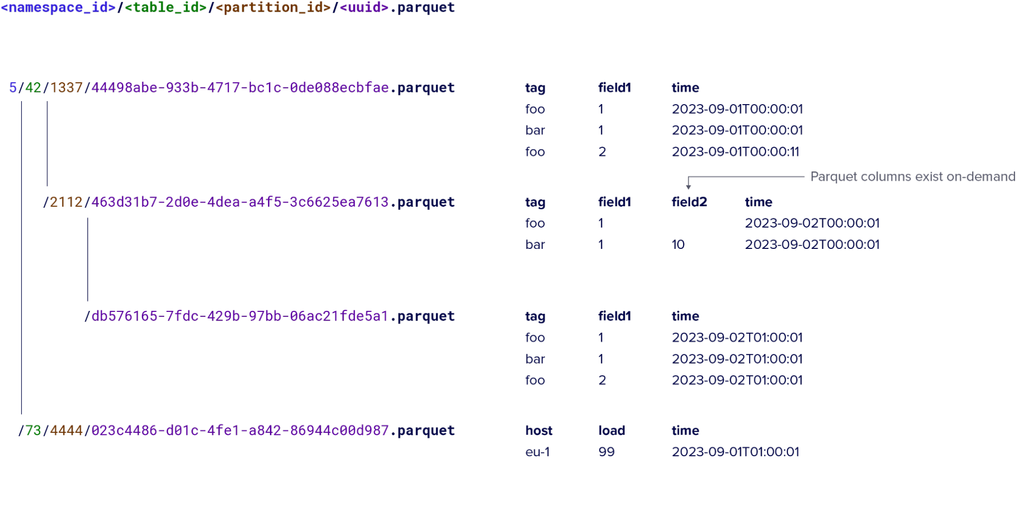
Parquet file partitioning and data model example for InfluxDB 3.0

InfluxDB 3.0 retains the notion of tags and fields; however, they play a different role in 3.0. A unique set of tag values and a time stamp identifies a row, which enables InfluxDB to update it with an UPSERT on write.

Now that we’ve explained a bit about the new data model, let’s turn to how it allows us to improve data ingest efficiency and compression.

Alternate partitioning options

We designed InfluxDB 3.0 to perform analytical queries (i.e. queries that summarize across a large number of rows) and optimized the default partitioning scheme for this. However, users may always need to query a subset of tag values for some measurements. For example, if every query includes a certain customer id or sensor id. Due to the way it indexes data and persists it to disk, TSM handles this type of query very well. This is not the case with InfluxDB 3.0 so those using the default partitioning scheme may experience a regression in performance for these specific queries.

The solution to this in InfluxDB 3.0 is custom partitioning. Custom partitioning allows the user to define a partitioning scheme based on tag keys and tag values, and to configure the time range for each partition. This approach enables users to achieve similar query performance for these specific query types in InfluxDB 3.0 while retaining its ingest and compression benefits.

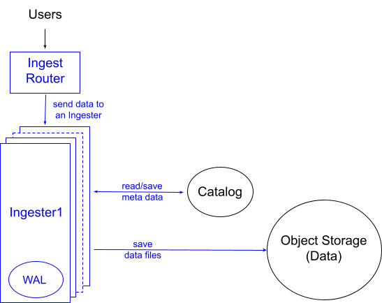
InfluxDB 3.0 ingest path

The data model for InfluxDB 3.0 is simpler than previous versions because each measurement groups all of its data together instead of separating it out by series. This streamlines the data ingest process. When InfluxDB 3.0 handles a write, it validates the schema and then finds the structure in memory for any other data for that measurement. The database then appends the data to the measurement and returns a success or failure to the user. At the same time, it appends the data to a write ahead log (WAL). We call these in-memory structures “mutable batches” or “buffers” for reasons that will be clear below.

This process requires fewer compute resources compared to other databases, including InfluxDB 1.x and 2.x because, unlike other databases:

1. The ingest process does not sort or otherwise order data; it simply appends it.
2. The ingest process delays data deduplication until persistence.
3. The ingest process uses the buffer tree as an index. This index lives within each specific ingester instance and identifies the data required for specific queries. We were able to make this buffer tree extremely performant using hierarchical/sharded locking and reference counting to eliminate contention.

Source

When the mutable batches run out of memory, InfluxDB persists the data in the buffers as Parquet files in object store. By default, InfluxDB will persist all the data into Parquet every 15 minutes if the memory buffer hasn’t been filled. This is the point where InfluxDB 3.0 sorts and deduplicates data. Deferring this work off the ‘hot/write path’ keeps latency and variance low.

Streamlining the ingest process in this way means that the database does less work on the hot/write path. The result is a process that moves operations that are expensive to execute to persist time so that overall it requires a minimal amount of CPU and RAM, even for significant write workloads.

From completeness, there is also a Write Ahead Log that is flushed periodically ensuring all writes are immediately durable, and is used to reconstitute the mutable batches in cases where the container fails. InfluxDB 3.0 only replays WAL files in unclean shutdown or crash situations. In the ‘happy path’, (e.g., an upgrade) the system gracefully stops, flushes (i.e., persists) all buffered data to object storage and deletes all WAL entries. As a result, startup is fast, because InfluxDB doesn’t have to replay the WAL. Furthermore, in non-replicated deployments, the data that would otherwise sit on the WAL disk on an offline node is actually in object storage and readable, preserving read availability.

Leading edge queries

We also optimized InfluxDB 3.0 for querying the leading edge of data. Most queries, especially time sensitive ones, query the most recently written data. We call these “leading edge” queries.

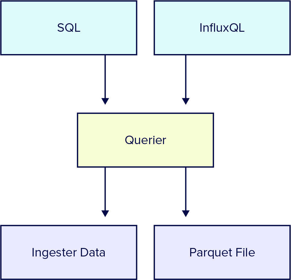
When a query comes in, InfluxDB converts the data to Arrow, which then gets queried by the DataFusion query engine. In cases where all the data being queried already exists in the mutable batches, the ingester serves the querier the data in arrow format, and then DataFusion quickly performs any necessary sorting and deduplicating before returning the data to the user.

In cases where some or all of the data is not in the read buffer, InfluxDB 3.0 uses its catalog of Parquet files – stored in a fast relational database – to find the specific files and rows to load into memory in the Arrow format. Once loaded into memory, DataFusion is able to quickly query this data.

Compaction

A series of compaction processes help maintain the data catalog. These processes optimize the stored Parquet files by ordering and deduplicating the data. This makes finding and reading Parquet files on disk efficient.

Data compression

There are a few key reasons why we selected the Apache Arrow ecosystem, including Parquet, for InfluxDB 3.0. These formats were designed from the ground up to support high performance analytical queries on large data sets. Because they’re designed for columnar data structures, they can also achieve significant compression. The Apache Arrow community, which we’re proud to be a part of and contribute to, continues to improve these technologies.

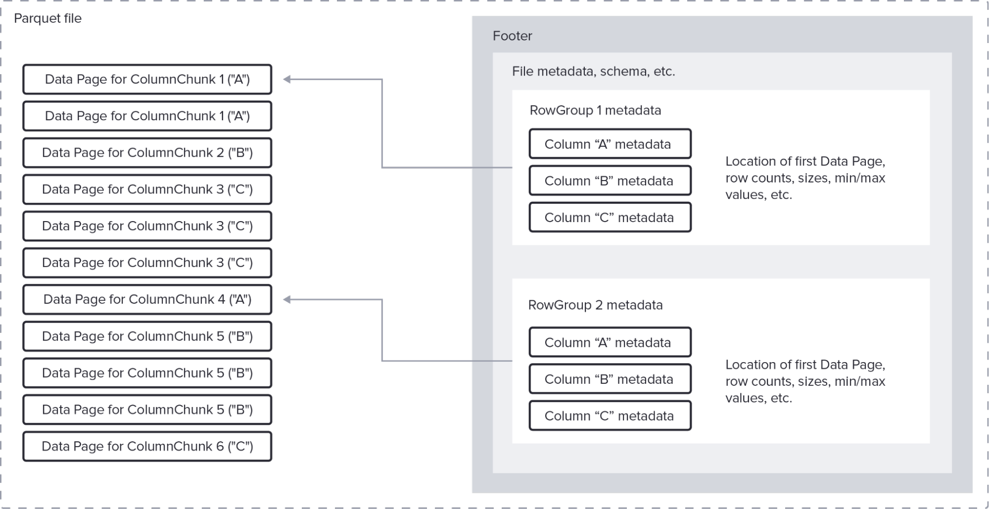Parquet file format

So, because InfluxDB 3.0 starts with Arrow’s columnar structure, it inherits significant compression benefits. Using Parquet compounds these benefits. Furthermore, because InfluxDB is a time series database, we can make some assumptions about time series data that allow us to get the most out of these compression techniques.

For example, suppose that retaining the notion of tag key/value pairs in InfluxDB 3.0 meant that dictionary encoding on these columns would yield the best compression. In this context, dictionary encoding assigns a number to each tag value. This number takes up a small number of bytes on disk. Then, Parquet can run length encode those numbers for each tag key column. On top of this encoding scheme, InfluxDB can apply general purpose compression (e.g., gzip, zstd) to compress the data even further.

The overall combination of Arrow and Parquet results in significant compression gains. When you combine those gains with the fact that InfluxDB 3.0 relies on object storage for historical data, users can store a lot more data, in less space, for a fraction of the cost.

Wrap up

Hopefully, you found this explanation of how InfluxDB 3.0 achieves such impressive ingest efficiency and compression interesting. In conjunction with the separation of compute and storage, customers can achieve significant total cost of ownership advantages over other databases, including InfluxDB 1.x and 2.x!

Try InfluxDB 3.0 to see how these performance and compression gains impact your applications.