IoT Prototyping with InfluxDB Cloud (Part 2): Queries, Tasks and Dashboards

By Rick Spencer / Use Cases, Product, Developer
Sep 27, 2019

This is Part 2 of a four-part series. Read Part 1, Part 3, and Part 4 as well.

The IoT scenario

Previously, I put together an IoT device (Prototyping IoT with InfluxDB Cloud - Part 1 of this series) and started streaming data to my InfluxDB Cloud account. It has been happily streaming data to my account since.

Next, I want to create a dashboard that shows changes in soil moisture levels over time, as well as the current soil moisture reading.

Smoothing the soil moisture reading

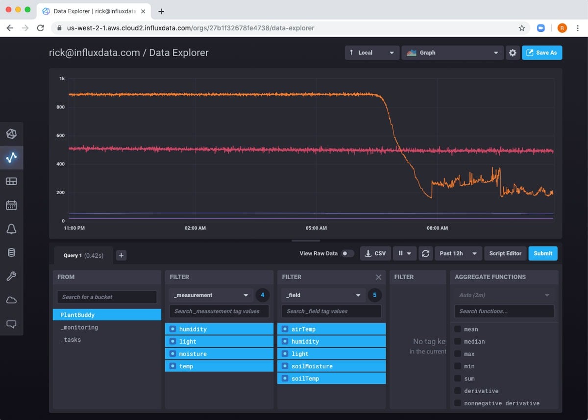
As you can see, the soil moisture reading can be a little jittery, and I would like to smooth this over a little. Additionally, my PlantBuddy bucket stores a reading for each sensor every 3 seconds. While this is very useful for certain types of analysis and functionality, storing all of this data long-term serves little value and will add to the expense of the project.

There are many ways to approach this. I am going to take a simple approach for a first iteration.

• I will create a new bucket to hold downsampled data.
• I will write a query that takes the last 5 minutes of data from the raw bucket, computes a mean, and puts this data into the new "compressed" bucket.
• I will create a task from this query that runs every five minutes.

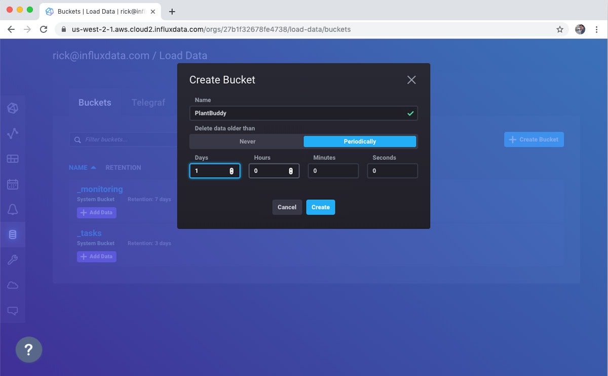
Create a new bucket

First I create a new bucket for holding the downsampled data. Note that I am still using a free tier account, so I can’t turn the retention up past 72 hours yet.

Use Flux to "compress" the data

Now I am going to write a Flux query in the Data Explorer to compress the data.

Introduction to Flux

In case you aren’t familiar, Flux is a new query language that is designed to be a general-purpose data transformation language. It was designed to be simple to use, but also powerful enough to handle any data transformation task.

Conceptually, Flux reminds me a bit of piping with awk. Essentially, you write a series of statements that takes a table of data as input, does some change to the table, and then outputs a new table to the next statement.

Flux has the following interesting combination of language characteristics:

• Flux is strongly and statically typed. This means that many errors can be caught right when you create them, but also you can get rich editor features, such as statement completion, inline help, etc.
• Flux does not require type specification when declaring variables. Though strongly and statically typed, Flux is able to infer types from context, so as when you are writing Flux code, you don't have to worry about types.
• Flux uses keyword arguments everywhere. This makes Flux code much easier to read and understand.

If none of that makes sense to you, or you just don’t care, that’s fine. It is probably easier to show than to explain.

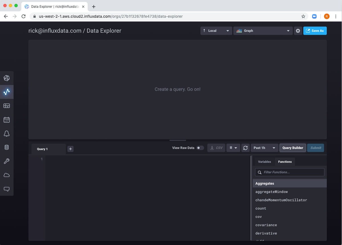
First, go to the Data Explorer View.

Then click “Script Editor” to switch to the Script Editor view.

Now I can interactively write some Flux. Generally, a Flux script will start with a “from” statement. This tells the script where to get the first table to work on. In this case, I want to get the table from the PlantBuddy bucket, because that is where all of the data is. “from” is a function, and functions in Flux use named parameters. So, I will tell my query to get the initial data from a bucket called “PlantBuddy” like this:

from(bucket: "PlantBuddy")

This should simply return a table with all of the data in the bucket. However, InfluxDB Cloud 2.0 does not support this because this is likely a TON of data to export, and is very unlikely what you meant to do. Note that this is not a limitation of the Flux language, per se, but is just in place to keep users from accidentally blowing out their usage quotas accidentally, and not taxing the database engine with accidental queries.

Therefore, it is necessary to add at least one pipe to limit the data to select. In Flux, you use the pipe forward operator (|>) to output a table to the next operation in the query. This is obviously similar to the pipe symbol in Unix systems. So, to start, I will ask InfluxDB for just the last 5 minutes of data from the bucket. I do this by “piping” the data in the bucket to the range function. The range function has start and end arguments. I will set “start” to “5 minutes ago” using the following notation:

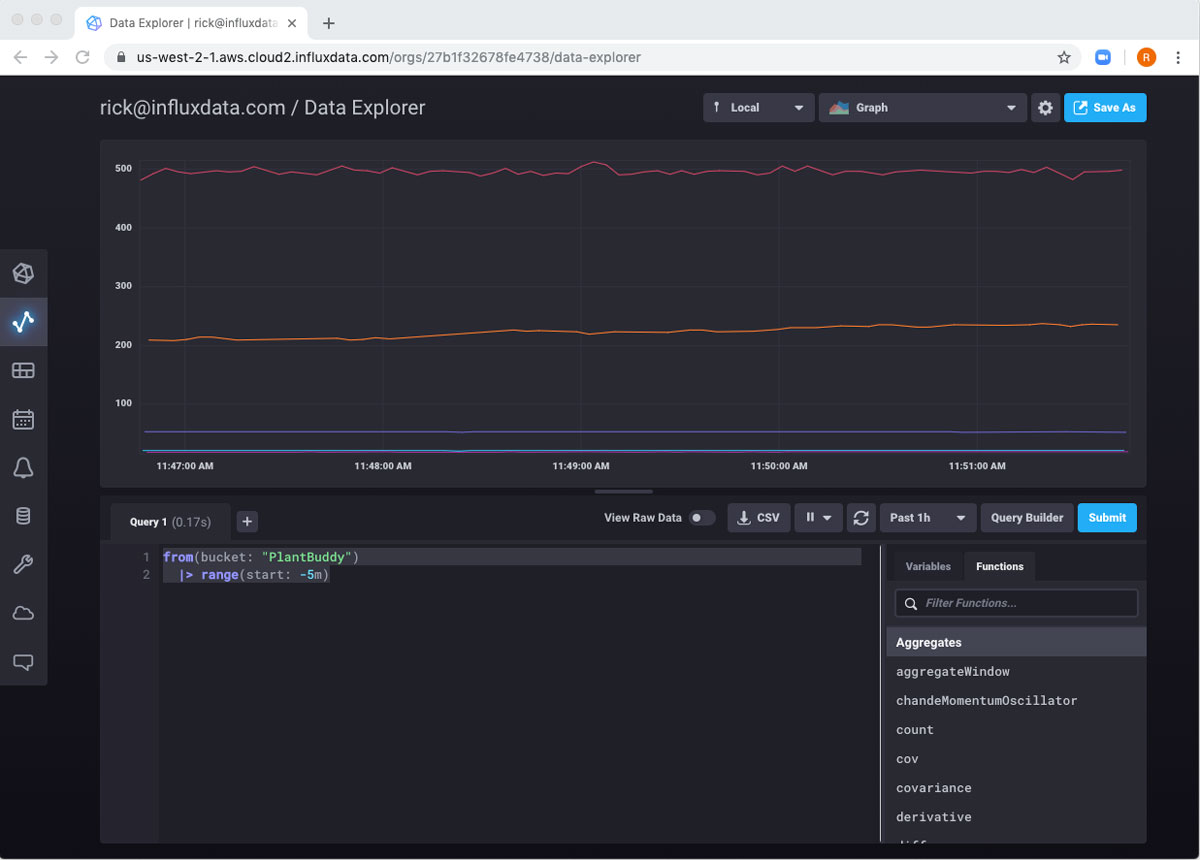
from(bucket: "PlantBuddy")
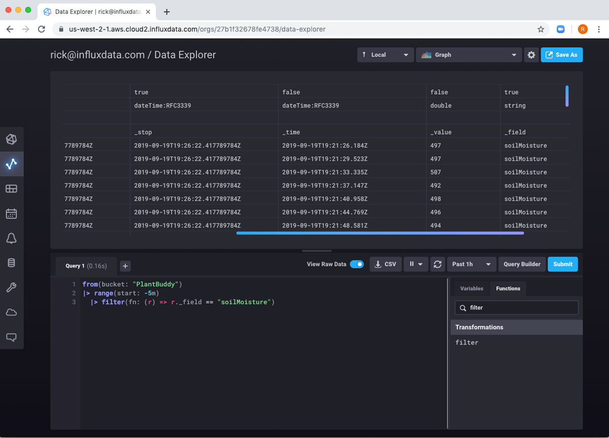
  |> range(start: -5m)

Now if I hit “submit”, I can see the last 5 minutes of data returned.

To make it easier to see the resulting table, I can switch to “Raw Data” view.

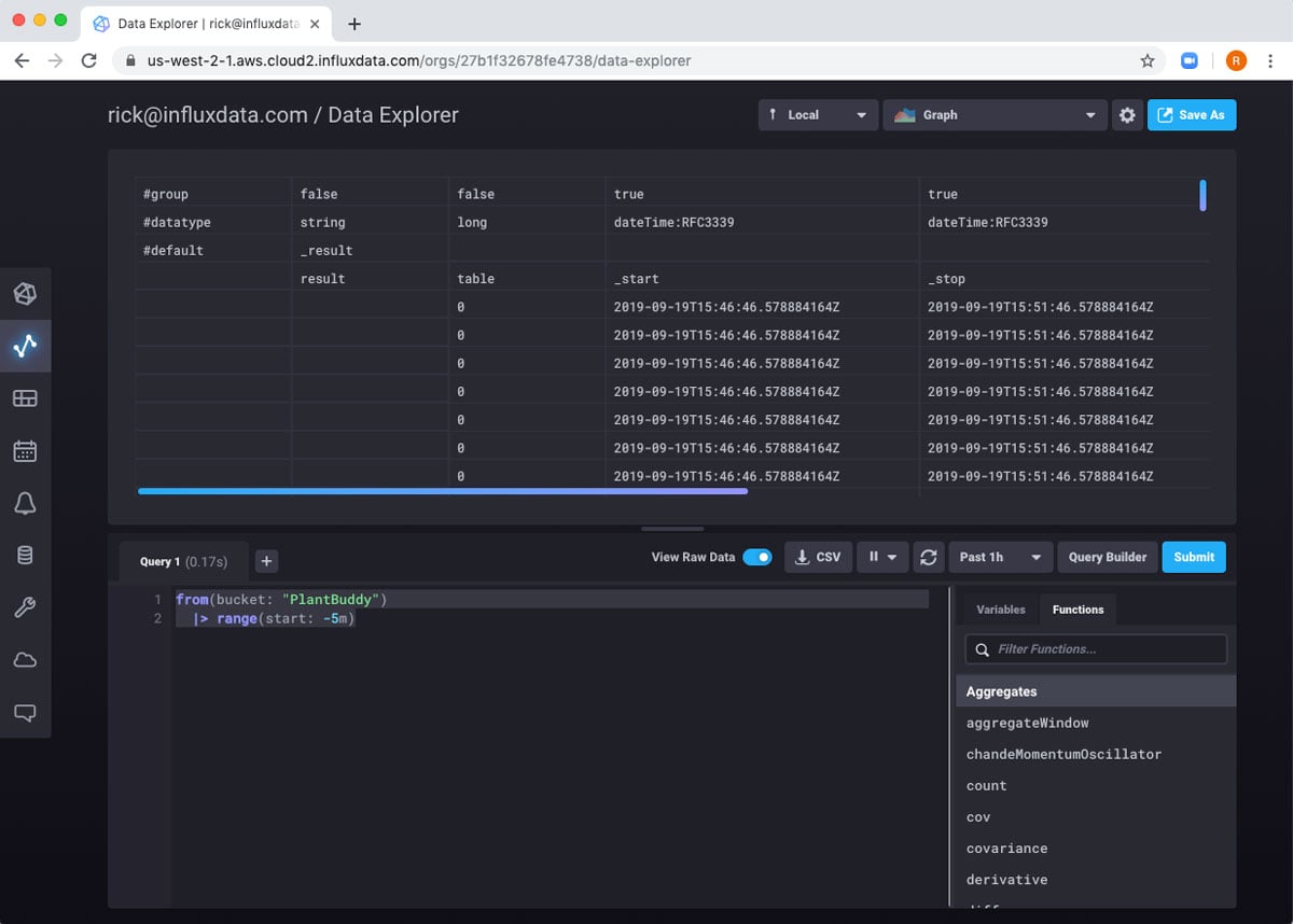
Now I can really see the data returned.

Flux includes functions for ordering the data, but I don’t particularly need that. However, I only want the soilMoisture readings. So I will pipe this table into a filter function. I can use the Functions list to get some help writing the function. It provides a stub implementation, and useful documentation right inside the Query Builder.

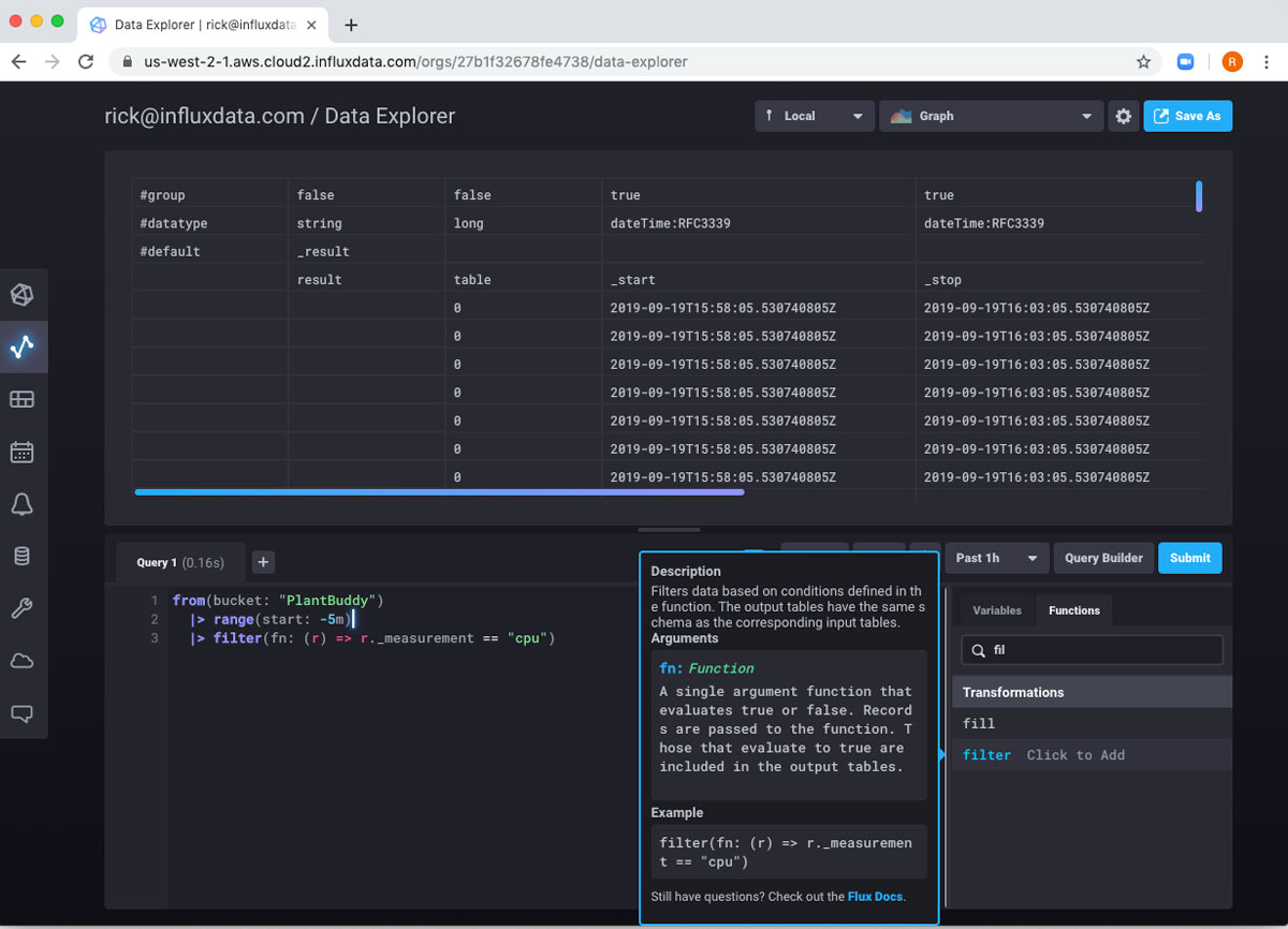
filter() is a function that takes another function as an argument. This pattern may be familiar to users of various JavaScript libraries. This should feel like creating an anonymous function if this is something you are familiar with. If not, don’t worry, it’s quite simple both conceptually and in practice.

Here is the line of Flux that does the filtering:

|> filter(fn: (r) => r._measurement == "cpu")

We can break this down a little to help understand it a little more. “filter” is the name of the function. filter() requires a named parameter called “fn” which is another function. This means I need to pass another function into the filter() function. The function that I pass in will do the actual filtering. “r” stands for “Record” and is an implicit variable that a row of the table is being passed into the the filtering implementation. The actual filtering is just a boring boolean expression. If it returns true, the record is kept. Otherwise, the record is tossed.

Of course, if I submit this query, I get no results because my device doesn’t measure any CPUs. What I care about is the soilMoisture readings, and those captured in rows where the field is called “soilMoisture.”

And we can see that this working. So, now I can add another pipe to calculate the mean of all of those fields. I can search for the function and get a little help.

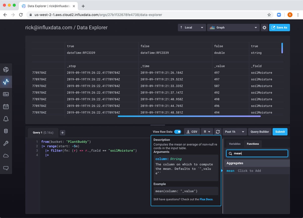
The mean function uses the _value field by default, which works for me, so I can just add that to my code:

from(bucket: "PlantBuddy")
|> range(start: -5m)
|> filter(fn: (r) => r._field == "soilMoisture")
|> mean()

Now when I submit that query, I get a single value in the table, the mean of all of the rows passed through the pipes so far.

I’m not quite ready to move it to my new bucket yet because the result of the mean() function removed the _time column and I will get an error if I try to add the result to the bucket without the _time column. The mean() function did add a _start column and a _stop column. I don’t need either of those, so I will simply use the rename() function to change the name of the _stop column to “_time”:

from(bucket: "PlantBuddy")
  |> range(start: -5m)
  |> filter(fn: (r) => r._field == "soilMoisture")
  |> mean()
  |> rename(columns: {_stop: "_time"})

And if I submit that, I can see that there is now a _time column.

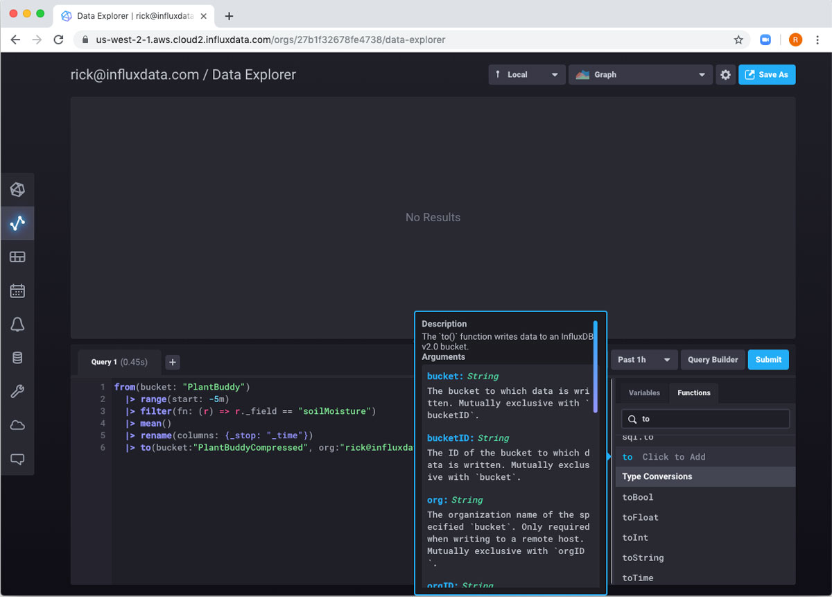
Now I just need to send it to my bucket. Since you get data into your Flux script using “from”, it only makes sense that you export it using “to”:

from(bucket: "PlantBuddy")
  |> range(start: -5m)
  |> filter(fn: (r) => r._field == "soilMoisture")
  |> mean()
  |> rename(columns: {_stop: "_time"})
  |> to(bucket:"PlantBuddyCompressed", org:"[email protected]")

When I submit this query, I get “No Results” because I sent all the data to the other bucket.

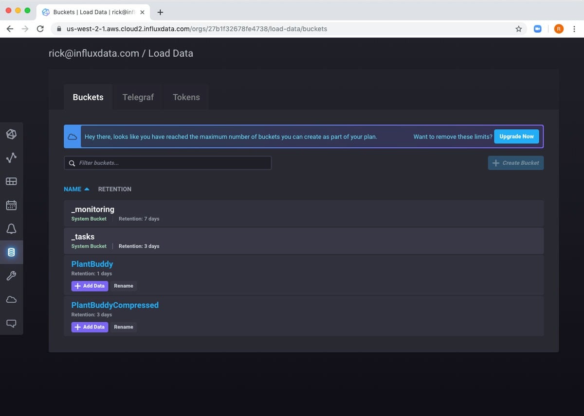
Since I only ran the task once, I know that there will only be a single row in the bucket. If I look at PlantBuddyCompressed, I can see that the single row is there.

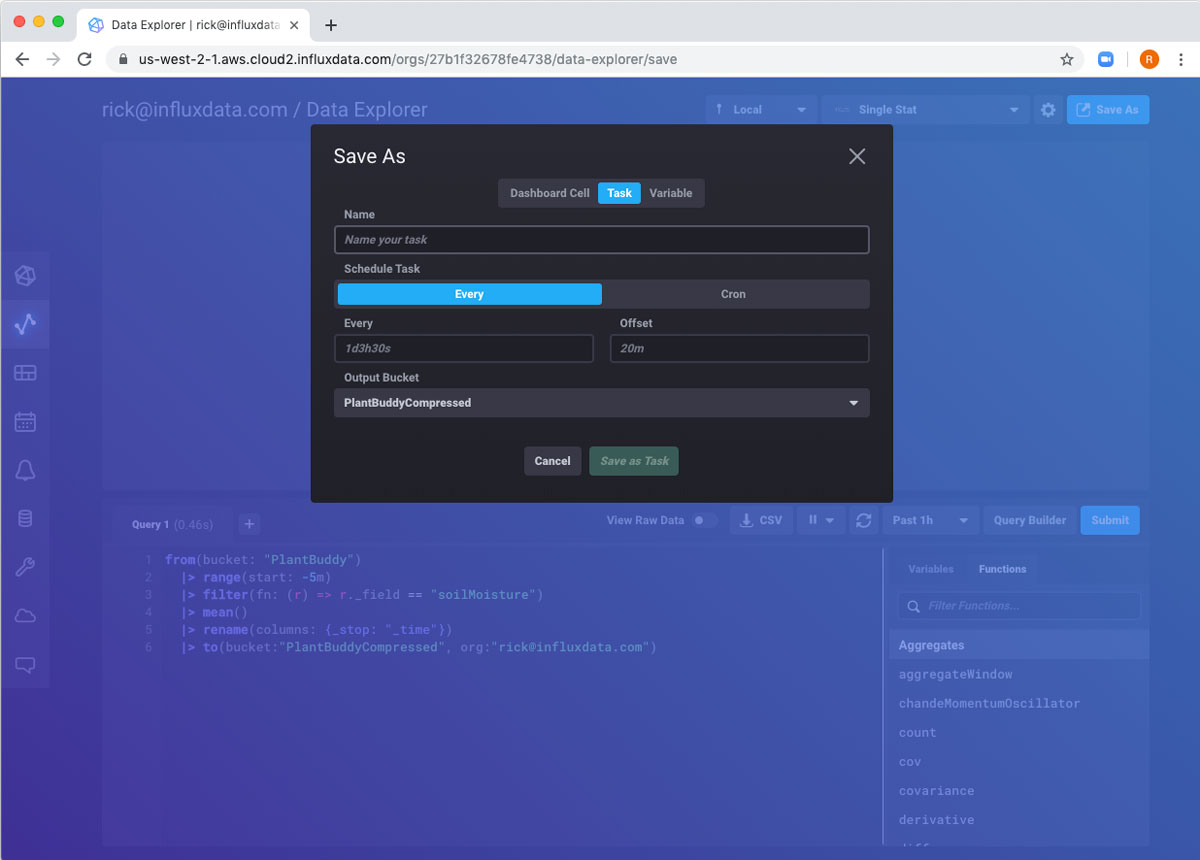
Creating a task from the query

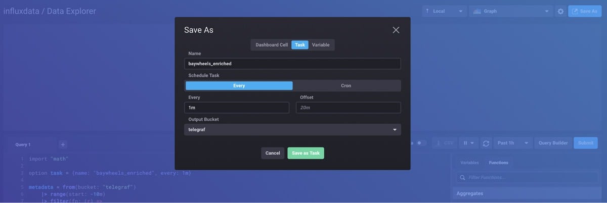
So now that I have a Flux query that is working well, how do I run it every five minutes? That’s exactly what tasks are for. The Save As button in the top right will let me convert the query into a task.

I just need to fill in a name for the task, and how often to run (in this case every 5 minutes).

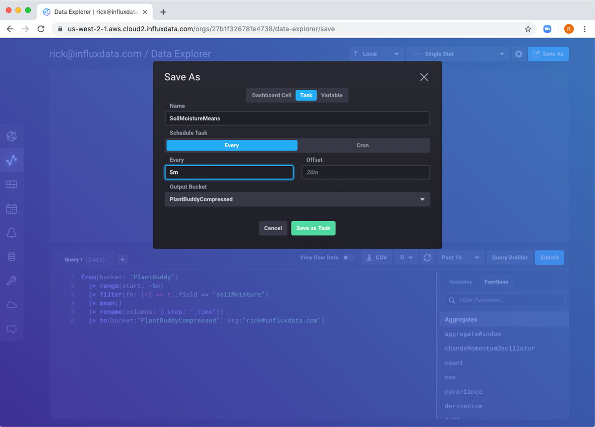
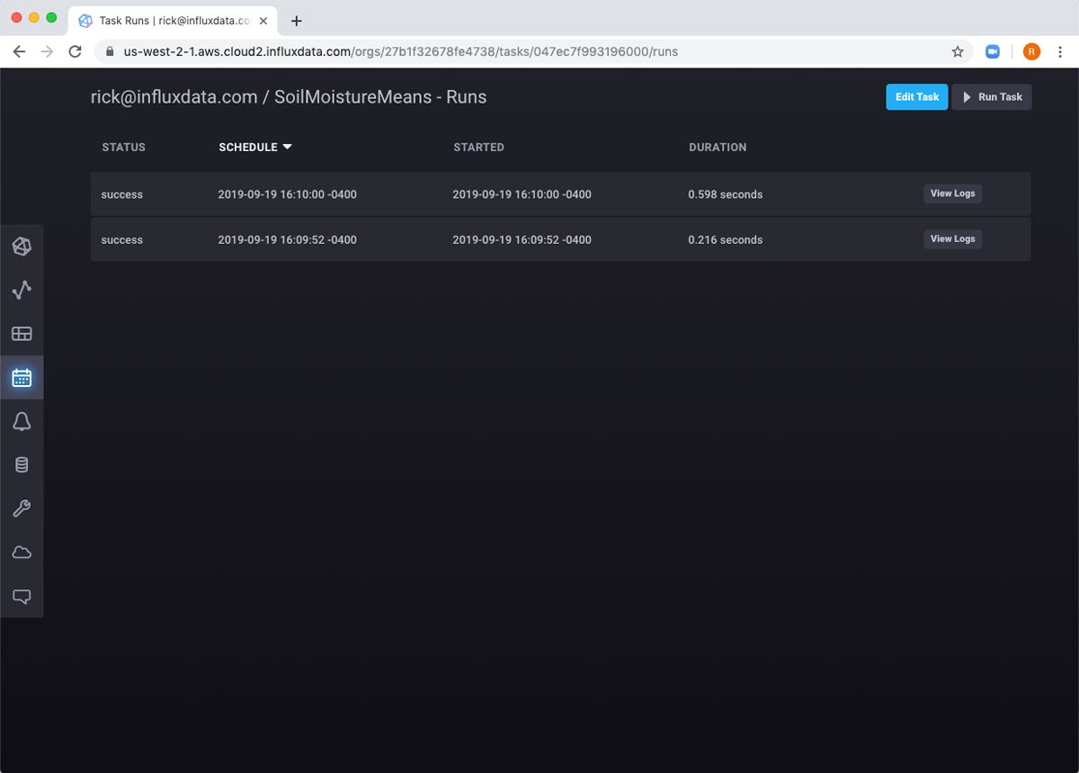
After completing the form, the task is created and I am taken to the task page automatically.

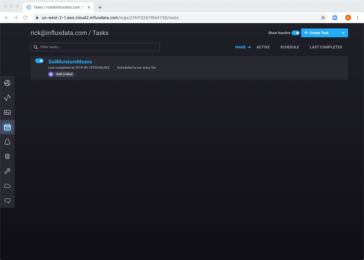
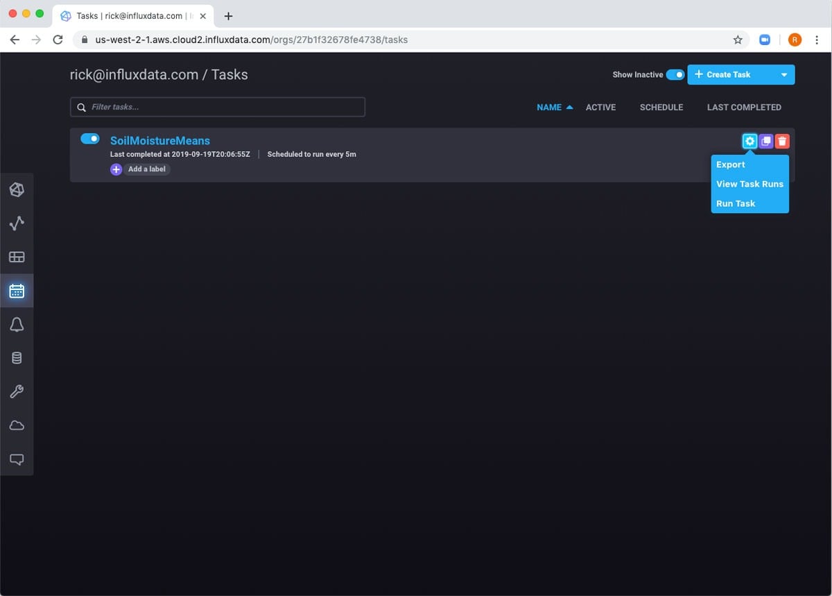
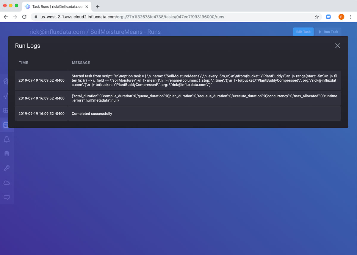
If I hover over the row, I can see some different ways I can interact with the task. For example, I can run the task manually, and then review the logs.

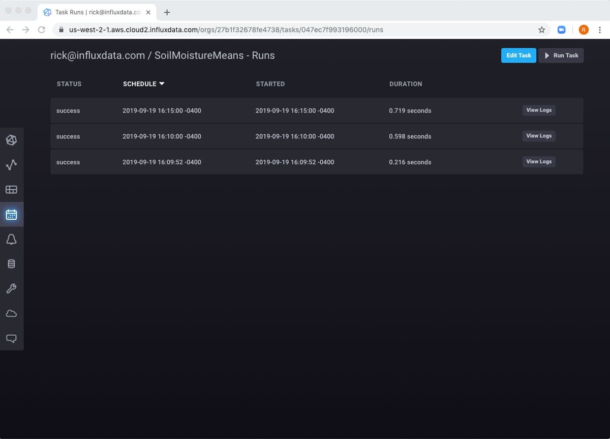
If I wait five minutes, I can see that the task has run again.

Create a dashboard

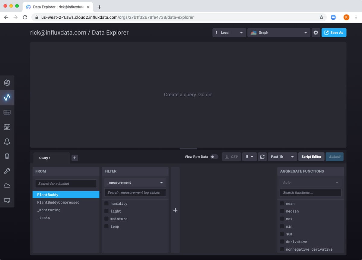
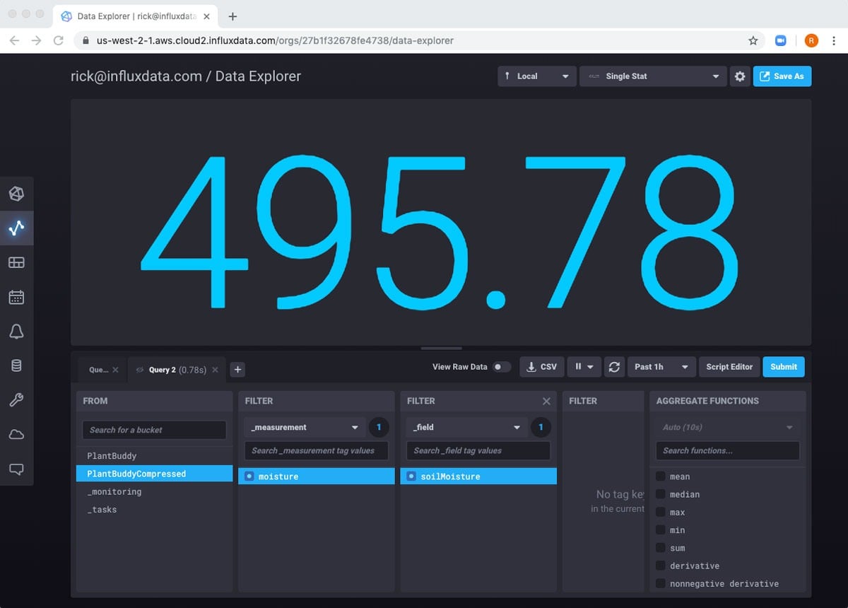
So, this is really great that I am running my task periodically and reliably. But what I would really like is a dashboard so that I can see at a glance how my plant is doing. To get started, I will go back to the Data Explorer so I can start working on a new query.

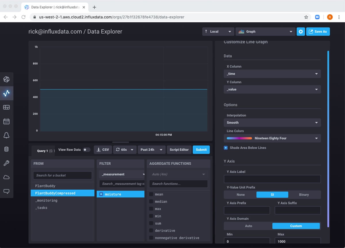
This time, I am interested in my new bucket, PlantBuddyCompressed, so I will select the soilMoisture Readings from there.

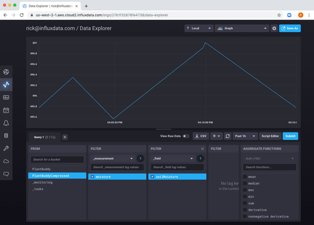
So, I can see my data, but the default view is not really perfect for my dashboard. I really want it to refresh automatically, and I want to see where the values are between the full possible range of 0 to 1000. In order to implement these, I will simply click the gear icon at the top right, and configure the chart the way I want, as well as set it to refresh every 60s.

Now, I want to export all of this to a dashboard. Once again, the Save As button at the top right will allow me to do this.

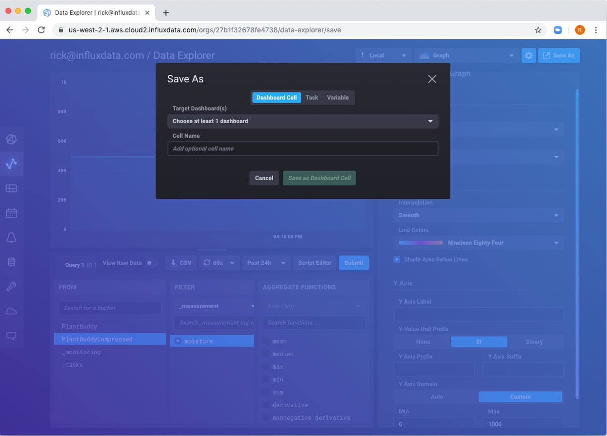
Because there are no existing dashboards, I need to use the dropdown to choose to create a new one. I fill in the form and save.

Now if I navigate to Dashboards in the left-hand nav, I can see my new Dashboard is created. And if I click on it, it looks like nothing is working.

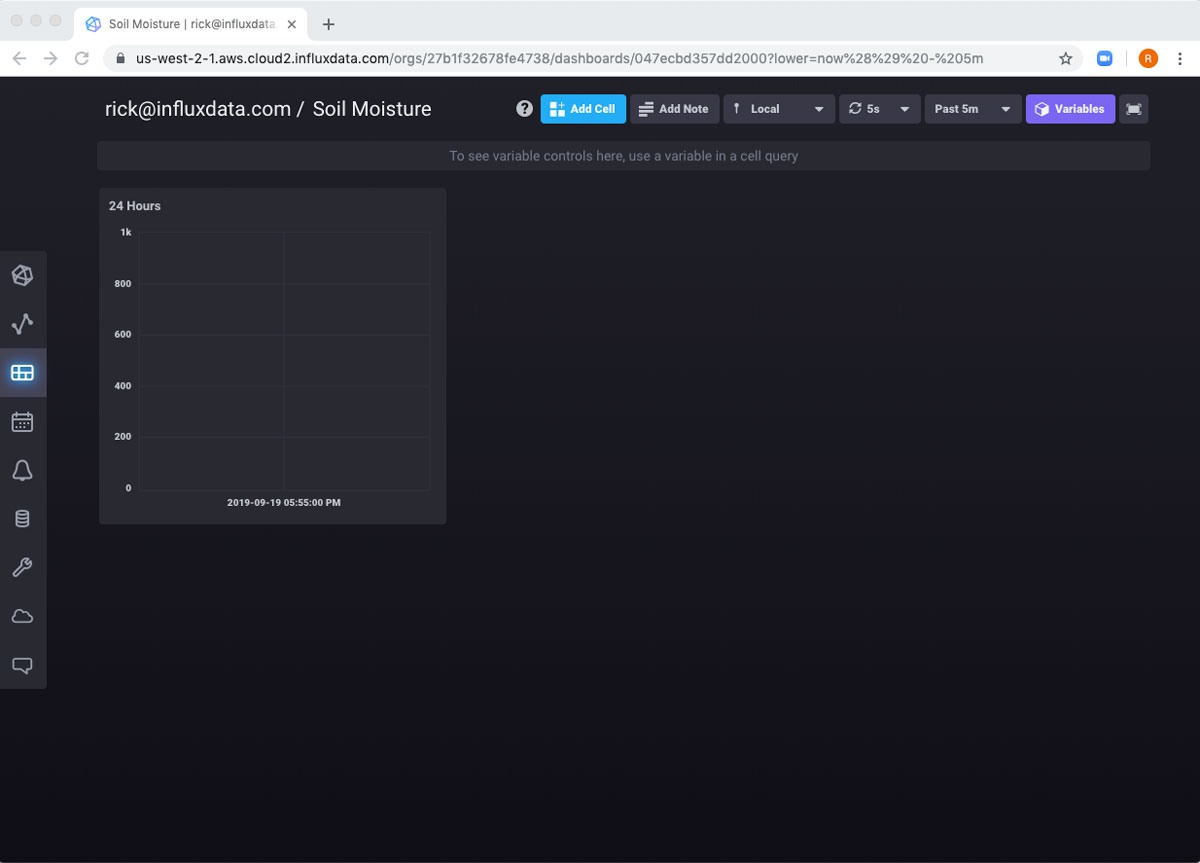
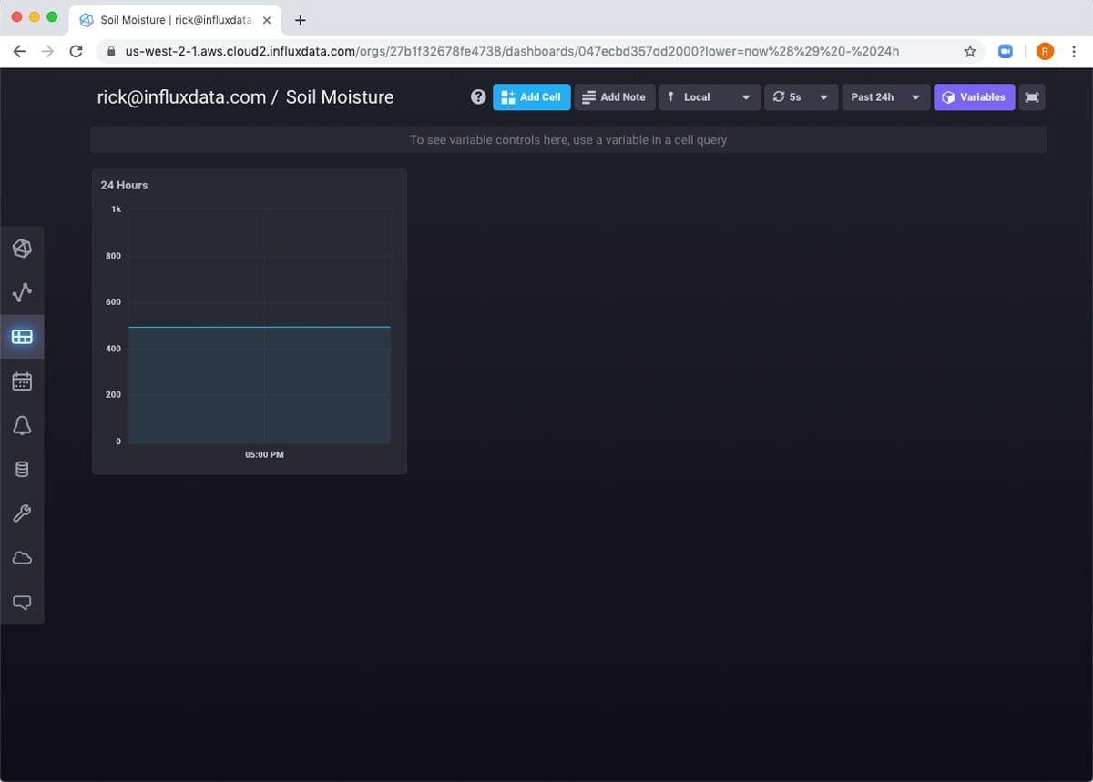
That’s only because the global scope at the top of the dashboard is set to 5 minutes. If I change it to 24 hours, it works.

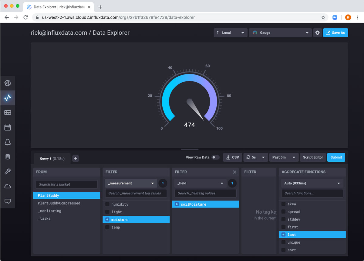
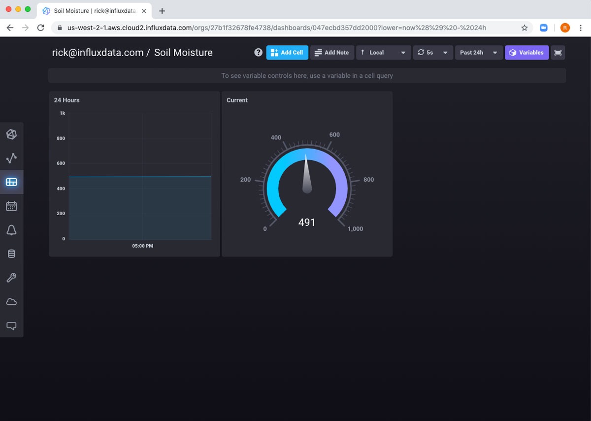
I want to add something else to the dashboard: the current soil moisture level. This I will grab from the uncompressed bucket. Since it’s a single number, I can use a gauge to visualize it.

I’ll change the range of gauge to be 0 to 1000.

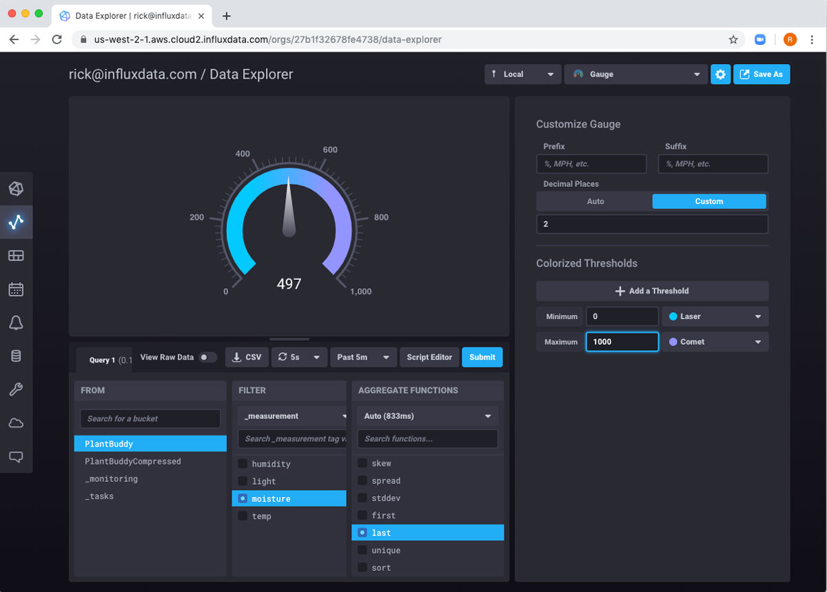
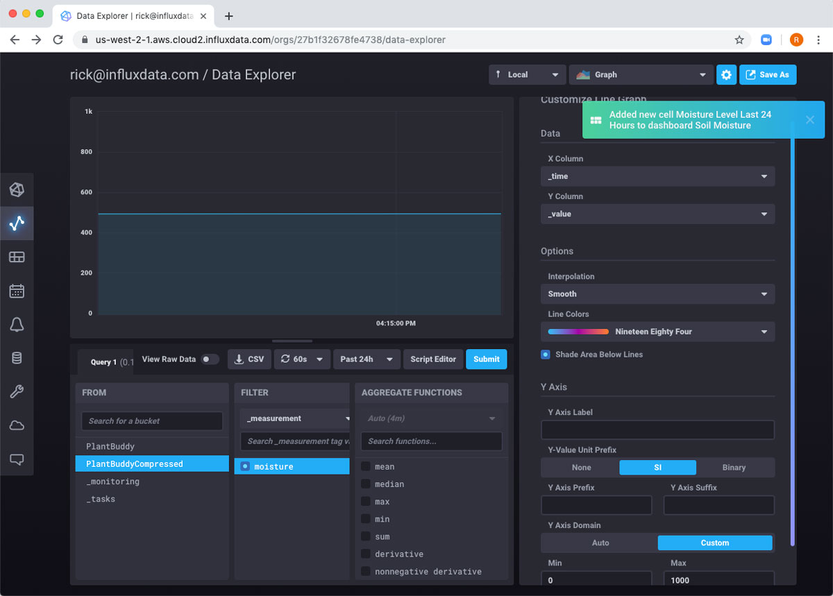
Then I will use the Save As button to create another dashboard cell. Now I have both cells on my dashboard, and I can keep a good eye on my plant!

Now that you’re done reading Part 2 of this series, go on to read Part 3.