Python ARIMA Tutorial 2026
By
Community
updated March 13, 2026
Developer
Navigate to:
Time series forecasting is an essential part of data analysis in fields such as finance, weather prediction, and sales forecasting, among others. The ARIMA model—a statistical method well known for its efficiency in estimating and forecasting time-dependent data—is a major topic in this domain. It is loved by many because it accurately models a variety of time series, making it a powerful tool in predictive analytics.
This guide will break down implementing ARIMA models in Python, a language with rich libraries and tools for data analysis. The simplicity and extensive support Python offers make it suitable for use with complex statistical models like ARIMA.
We’ll start by setting up your Python environment and building, evaluating, and optimizing ARIMA models. By the end of this post, you should be able to grasp the ARIMA model clearly and understand how to apply it for effective forecasting with Python.
What is ARIMA?
The AutoRegressive Integrated Moving Average (ARIMA) is a fundamental tool in time series analysis. It examines past values to understand and predict points within a data sequence. This model is particularly useful when dealing with data that changes over time. It consists of three key parts:
1. AutoRegression (AR)
This represents how much one variable depends on previous variables. AR estimates future values based on past observations; it looks at the relationship between a variable and its prior values.
2. Integration (I)
These are contrary operations that remove trends or seasonality from the data so that their mean and variance are constant over time. Basically, this means differencing the data (i.e., subtracting the previous value from the current value).
3. Moving Average (MA)
This incorporates errors that occurred previously, taking a combination of past errors into account while modeling them. It can be used to mitigate data noise and identify its underlying trend.
ARIMA parameters (p, d, q)
- p denotes the AutoRegressive order. That is the number of lags in a model. For example, if p = 2, then the model uses two previous time points to predict the current value.
- d is the degree of differencing required to make the data stationary (one with a constant mean and variance over time). Say d=1, then you’ll subtract the previous value from the current at least once; otherwise, if d = 0, then the data is stationary.
- q shows the order of the moving average, which is the residual errors on MAs applied to lagged observations.
When to use ARIMA
The ARIMA model is widely applicable in real-life scenarios. As a result, it is ideal for modeling data with trends and seasonality, such as:
- Economic forecasting: Predicting GDP, unemployment rates, or stock prices
- Sales forecasting: Forecasting future product demand based on previous sales data
- Weather forecasting: Temperature, rainfall, or other weather condition predictions
- Resource allocation: Forecasting inventory or production needs in industries such as retail and manufacturing
Python offers a range of libraries for implementing ARIMA, such as statsmodels, which provides numerous features for building and analyzing models. Thus, Python is an effective tool for learning about ARIMA models and practically applying them.
Prerequisites
Here’s what you’ll need to follow along with this tutorial:
Basic Knowledge
- Python proficiency: Familiarity with basic Python programming
- Statistical understanding: Fundamental aspects of statistics, especially relevant to time series data
Tools and Libraries
- Python: The primary language for implementation
- Jupyter Notebook: An interactive coding experience
- Key libraries: pandas, NumPy, matplotlib, statsmodels (pip installable)
Setting up your environment for ARIMA in Python
Installing Jupyter Notebook
- Open the command line or terminal: Go to the command line (Windows) or terminal (Mac/Linux).
- Install Jupyter: Type pip install notebook and press enter to install Jupyter Notebook on your computer.
Installing Python libraries
The following steps guide you through installing the Jupyter Notebook. To open the Jupyter Notebook, type jupyter notebook in your command line or terminal and press enter, as mentioned below.
- Create a new notebook: In the Jupyter interface, create a new notebook for your ARIMA project.
- Install libraries in notebook: Type and run the following commands in separate cells:
- !pip install pandas for data manipulation
- !pip install numpy for numerical operations
- !pip install matplotlib for data visualization
- !pip install statsmodels for statistical modeling, including ARIMA
These steps ensure you have a functional Python environment with all the necessary tools to start working with ARIMA models.
Implementing your first ARIMA model in Python
Importing Necessary Libraries
Start by importing the libraries you’ll need. In your Python environment (such as a Jupyter Notebook), enter the following commands:
import pandas as pd
import numpy as np
import matplotlib.pyplot as plt
from statsmodels.tsa.arima.model import ARIMA
from statsmodels.tsa.stattools import adfuller
Loading and Visualizing Time Series Data
We’re going to use this data from Kaggle.
- Load data: Use pandas to load your time series data. For instance, you can use data = pd.read_csv(‘data.csv’).
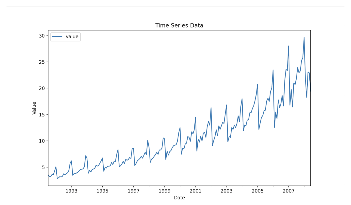
- Visualize data: Plot your data to understand its pattern. Here’s an example:
data.plot()
plt.show()
Testing for Stationarity
Stationarity is crucial for ARIMA models. Use the augmented Dickey-Fuller test to check for stationarity:
result = adfuller(data['column_name'])
print('ADF Statistic: %f' % result[0])
print('p-value: %f' % result[1])
If p-value > 0.05, the data are non-stationary and require differencing.
Differencing If Necessary
If your data is non-stationary, difference it:
data_diff = data.diff().dropna()Determining ARIMA Parameters (p, d, q)
- Plotting: Use plots (like autocorrelation and partial autocorrelation plots) to estimate ‘p’ and ‘q’.
- Statistical tests: Use statistical methods or rules of thumb to find optimal ‘p’, ‘d’, ‘q’ values.
Building and Fitting an ARIMA Model
Create and fit an ARIMA model with your chosen parameters (here we’ve chosen 1 for all parameters):
model = ARIMA(data_diff, order=(1,1,1))
model_fit = model.fit()
Making Predictions
Use the fitted model to make forecasts:
predictions = model_fit.forecast(steps=5)  # Predict next 5 points
print(predictions)
Check Residuals
Plot to see the distribution of residuals:
model_fit.plot_diagnostics(figsize=(10,6))
plt.show()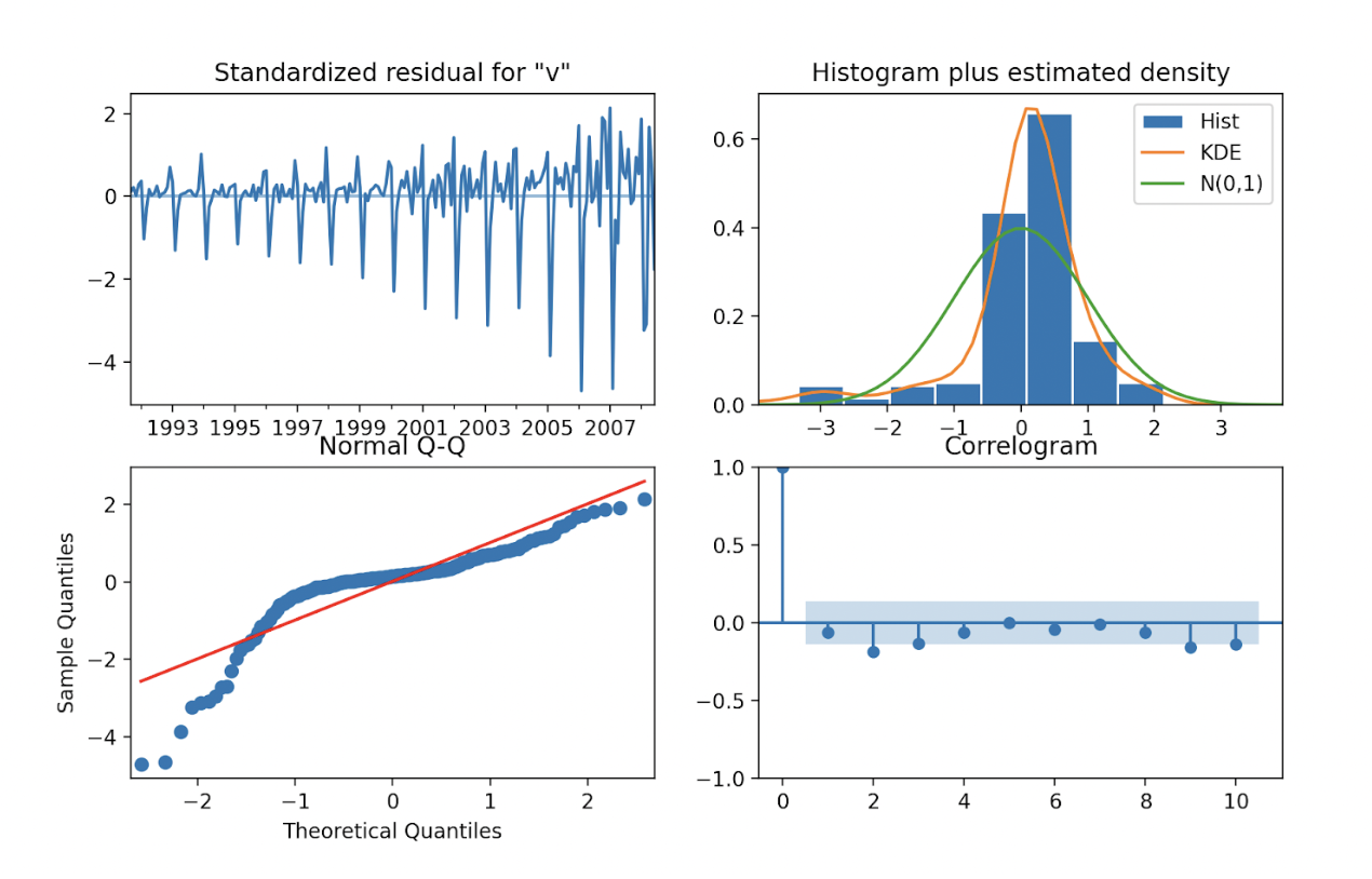
How to evaluate an ARIMA model
Once you have programmed the ARIMA model in Python, it’s essential to evaluate its performance. Knowing how well your model fits the data aids in precise forecasting.
Understanding Performance Metrics
- Akaike Information Criterion (AIC): This is a measure of how good a model is. It evaluates the relationship between the model’s complexity and how well it fits the data. The best value for AIC is minimal.
- Bayesian Information Criterion (BIC): Similar to AIC, this method assesses quality but penalizes complex models more strongly than AIC. The best value for BIC is minimal.
- Root Mean Square Error (RMSE): This metric gives an average error size. It is derived by taking the square root of mean-squared differences between the prediction and the actual observation in cases where a lower rise implies better.
Interpreting the Model Summary
You can find a summary of the ARIMA model in the statsmodels library. These are some critical things to look at:
- Coefficients: The importance of each feature relative to the dependent variables is revealed by these values.
| Metric | Meaning |
|---|---|
| P > z | (p-values): Low p-values (usually < 0.05) imply that the parameters in this model are statistically significant. |
- AIC/BIC values: Use these to compare models.
Tuning your ARIMA model
To enhance forecasting accuracy, an ARIMA model needs its parameters (p, d, q) fine-tuned. The following are the appropriate steps to take.
Fine-Tuning Model Parameters (p, d, q)
- Iterative approach: Test different combinations of p, d, and q based on initial analysis (such as ACF and PACF plots). For each combination, monitor the model’s performance and adjust accordingly.
- Understand the data: Sometimes, through analyzing data, we get an idea of how much differencing is required (d) or the number of lag values to be included (p and q).
- Simplicity matters: A simpler model that does well with fewer values of p, d, and q is often better than a complex one. Too many parameters result in overloading results.
Grid Search for Parameter Optimization
Grid search is the hand-specified examination of an entire space of hyperparameters. The main aim is to find the combination of p, d, and q that minimizes a metric or score.
Implementing Grid Search in Python
Here’s a simplified example of how to implement grid search for ARIMA model parameters in Python:
from statsmodels.tsa.arima.model import ARIMA
import itertools
# Define the p, d, and q ranges to try
p = range(0, 3)
d = range(0, 2)
q = range(0, 3)
pdq = list(itertools.product(p, d, q))
best_score, best_cfg = float("inf"), None
for param in pdq:
    try:
        model = ARIMA(train_data, order=param)
        model_fit = model.fit()
        # Adjust this to use your preferred metric (e.g., AIC)
        if model_fit.aic "" best_score:
            best_score, best_cfg = model_fit.aic, param
    except:
        continue

print('Best ARIMA%s AIC=%.2f' % (best_cfg, best_score))
The code will test different combinations of p, d, and q and identify the one with the smallest AIC (in case you prefer another criterion). Keep in mind that optimization may require considerable computer time when working with larger datasets and many possible parameter combinations.
ARIMA in Python: wrapping up
We’ve now walked through developing, implementing, and debugging the ARIMA model in Python. Like any worthwhile journey, there were tricky turns along the way, but the knowledge you received in the time series prediction arena is priceless.
Keep experimenting and learning from your data. Each dataset has a narrative, and you are now better placed to reveal these concealed stories. Have a great time forecasting!
This post was written by Keshav Malik, a highly skilled and enthusiastic security engineer. Keshav has a passion for automation, hacking, and exploring different tools and technologies. With a love for finding innovative solutions to complex problems, Keshav is constantly seeking new opportunities to grow and improve as a professional. He is dedicated to staying ahead of the curve and is always on the lookout for the latest and greatest tools and technologies.
