Top 5 Hurdles for Flux Beginners and Resources for Learning to Use Flux

By Anais Dotis-Georgiou / Product, Use Cases, Developer
Dec 16, 2020

Are you new to InfluxDB v2.0 and Flux? Are you intimidated by learning a new time series scripting and query language? Perhaps you’re an InfluxDB v1.x user and you’re familiar with InfluxQL, and you’re unconvinced that learning Flux is worth your while? Or maybe you missed the Top 10 Hurdles for Flux Beginners session at InfluxDays North America 2020?

This two-part blog series aims to demonstrate the power of Flux and walk you through solutions to the top hurdles for both new and old InfluxDB users:

• The first post (the current one you're reading) introduces some of the most common hurdles for Flux beginners.
• The second post introduces some additional hurdles for intermediate Flux users.

Before we dive into Flux, let’s take a second to introduce it. Flux is a functional query and scripting language which was initially made available starting with InfluxDB v1.8+ and it is the primary language supported within InfluxDB v2.0 and Cloud. It is open source and JavaScript-esque. While the v2.0 API supports InfluxQL via backward compatibility, the power offered by Flux for working with data is substantial. A simple query might look like this:

from(bucket:"example-bucket")
  |> range(start:-1h)
  |> filter(fn:(r) =>
    r._measurement == "my-measurement" and
    r.my-tag-key == "my-tag-value"
  )

Query data from a bucket with the from() function. A bucket, for those new to this concept, combines the database and a retention policy concepts from InfluxDB v1.x . Retention policies determine how quickly time series data is expired and each bucket has a single retention policy within InfluxDB v2.x.

I like to picture a literal stream of time series data flowing into a bucket. The size of my bucket is equivalent to the duration of my retention policy. As time passes, the bucket becomes full and old time series data expires. 

In terms of getting familiar with Flux:

• Use pipe forward (|>) operators to apply an additional data transformation on your data.
• Use the range() function to query data for a particular time from that bucket.
• Use the filter() function to filter for particular measurements, fields, and tags.

Hurdle 1: Overlooking UI tools which facilitate writing Flux

This hurdle is important because it highlights the advantages of using the InfluxDB UI, and the solution exposes tools within the UI that you might not be aware of. This hurdle will be referenced multiple times throughout this post, and I encourage you to keep the UI at the forefront of your mind when trying to learn Flux.

Solution 1: Using the InfluxDB UI

InfluxDB v2.0 is a mature and unified product. To learn how to write Flux, you really want to learn how to use the InfluxDB native UI and vice versa. The UI is designed to enable you to create Flux scripts, tasks, and alerts without writing any Flux yourself. The most useful part of the InfluxDB UI for learning how to write Flux scripts is the Data Explorer. Within the Data Explorer, you have access to two Flux writing tools: Flux Query Builder and Flux Script Editor.

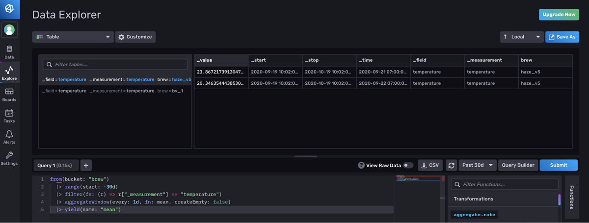
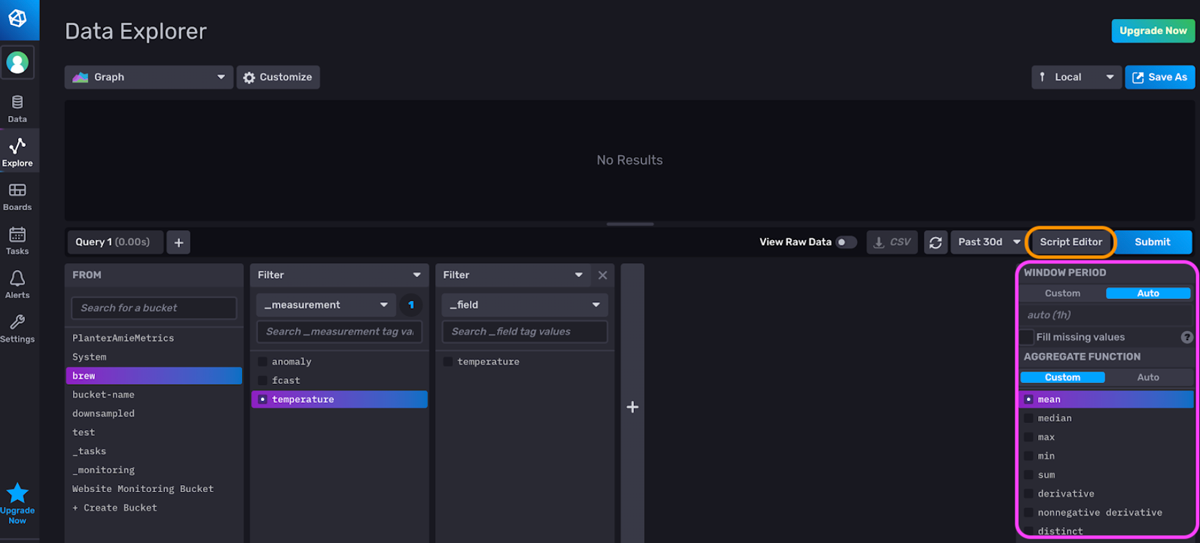<figcaption> The Flux Query Builder. Apply aggregation functions in the panel on the right (pink). Click on the Script Editor button (orange) to switch between the Flux Query Builder and the Flux Script Editor.</figcaption>

The Flux Query Builder allows you to:

• Visually create an underlying Flux script
• Select data from a bucket for a specific time range
• Apply filters on measurements, tags, and fields
• Apply an aggregation function

It’s worth noting that the Flux Query Builder applies an aggregation function by default. This aggregation is applied to reduce query time for queries with large read volumes and to enhance the visualization of your query. When querying large amounts of time series data, it’s usually more helpful to see a smoothed version of your dataset that accurately encapsulates the general trends of your data than the raw data. An aggregation provides the former. That being said, users are not always aware of the panel on the right that is applying an aggregation function. If you want to see your raw data, switch over to the Flux Query Builder and delete the aggregation function from your script.

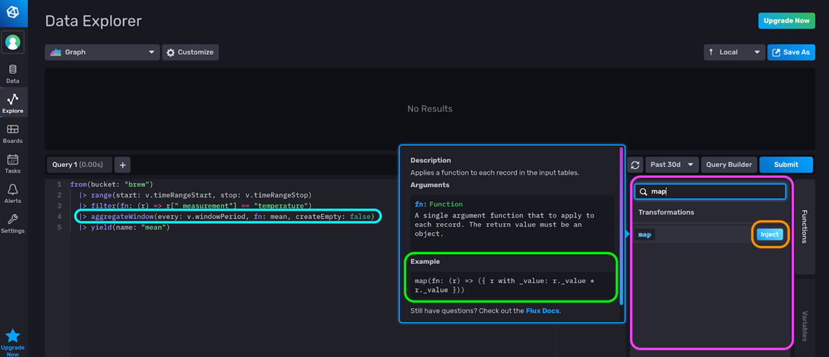<figcaption> The Flux Script Editor. The result is the corresponding Flux script for the output generated by the Flux Query Builder above. Search and inject functions in the panel on the right (pink). The Inject button injects the Example (green). By default, an aggregateWindow() function is applied to your data with the Query Builder (blue).</figcaption>

The Flux Script Editor allows you to:

• See the Flux Script produced by your selections in the Flux Query Builder
• Write your own Flux Script
• Filter for Flux Functions, inject functions into your Flux Script, and view in-app documentation about those Functions

I almost never write Flux by hand. Instead, I filter for the function I want to use, inject it, and alter it as needed. I encourage you to try the same approach.

Hurdle 2: Misunderstanding Annotated CSVs and sometimes writing them incorrectly

Understanding Annotated CSVs, the output format of InfluxDB v2.0, isn’t a trivial task. It can be tricky to wrap your mind around the way that data is structured in InfluxDB v2.0. I’ll also be the first to admit that this is especially true if you’re coming from InfluxQL or SQL. However, once you understand the output format of InfluxDB and how Flux operates on Annotated CSVs, then Flux really begins to click. After you cross that bridge, I genuinely believe that you’ll be happy with where you land. Every time I try to write complex queries with InfluxQL, I get frustrated. InfluxQL subqueries are hard to read and write compared to Flux. Take a look at From Subqueries to Flux for some evidence of that.

Solution 2: Understanding Annotated CSVs and using the array.from() function, to() function and universe directory in the Flux repo

To understand Annotated CSVs in detail, see How to Interpret Annotated CSVs. However, let’s briefly review here. Let’s assume our schema looks like this:

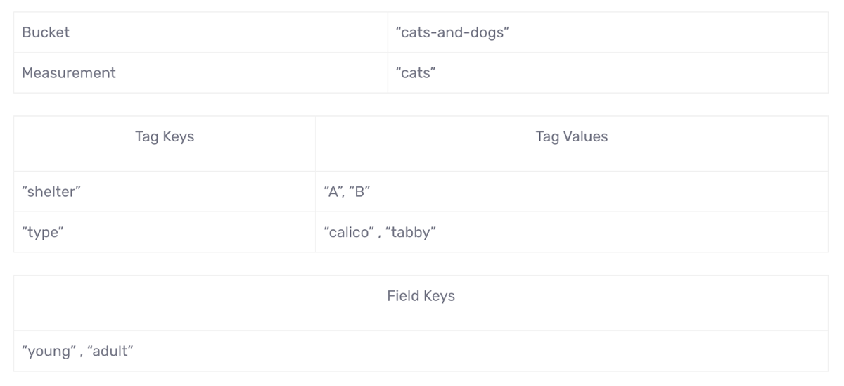
Then we might use the following Flux Query to find the number of adult calico cats in shelter A:

from(bucket: "cats-and-dogs")
 |> range(start: 2020-05-15T00:00:00Z, stop: 2020-05-16T00:00:00Z)
 |> filter(fn: (r) => r["_measurement"] == "cats")
 |> filter(fn: (r) => r["_field"] == "adult")
 |> filter(fn: (r) => r["shelter"] == "A")
 |> filter(fn: (r) => r["type"] == "calico")
 |> limit(n:2)

The corresponding Annotated CSV would look like this:

#group,false,false,true,true,false,false,true,true,true,true
#datatype,string,long,dateTime:RFC3339,dateTime:RFC3339,dateTime:RFC3339,double,string,string,string,string
#default,_result,,,,,,,,,
,result,table,_start,_stop,_time,_value,_field,_measurement,shelter,type
,,0,2020-05-15T00:00:00Z,2020-05-16T00:00:00Z,2020-05-15T18:50:33.262484Z,8,adult,cats,A,calico
,,0,2020-05-15T00:00:00Z,2020-05-16T00:00:00Z,2020-05-15T18:51:48.852085Z,7,adult,cats,A,calico

The first three lines with hashtags are annotations. The annotations contain metadata about our time series. I suggest focusing on the first two annotations. The first annotation, the group annotation describes which columns are part of a group key. A column is part of a group key when all the rows in that column are the same. In our example query above, we’ve filtered by a single field type, “adult”; a single “shelter” tag, “A”; and a single “type” tag, “calico”. These values are constant across rows, so those columns are set to true. Therefore, they are also part of the group key.

Understanding the Annotated CSV allows you to more deeply understand how Flux is transforming your data. Use the Raw Data View toggle between your visualization and the Annotated CSV output. Some people prefer looking at the Table visualization to debug their Flux. Both views can be helpful for understanding Flux. I think the preference between the Table visualization and Raw Data View is largely personal. However, I prefer inspecting the Raw Data View to debug my Flux script.

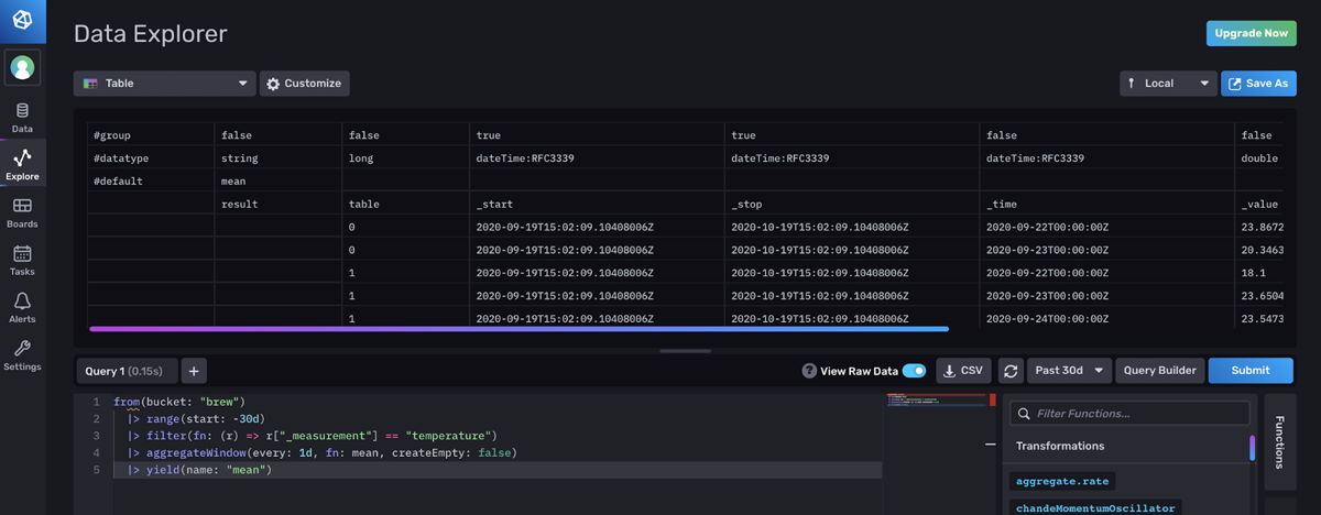<figcaption> The Raw Data View. Both tables are visualized in one pane.</figcaption>

I prefer the Raw Data View because it consolidates all of the tables in a single panel. By contrast, you have to click between tables in the Table visualization to look at all of your data.

<figcaption> The Table visualization. Tables are separated. Search for and switch between tables by selecting a table in the panel on the left.</figcaption>

Additionally, I find the metadata in the Annotated CSV in the Raw Data View extremely useful. For example, you might need to make sure that you have the correct data type when performing math on a certain column. Also, the group key annotation allows you to understand the shape of your data at a glance. I find the single pane view easier to work with than cross-comparing the shape of and content across a large collection of tables.

The array.from() and to() functions are necessary tools in your Flux toolbelt. With them, you can easily write data to InfluxDB. I find that creating dummy data with array.from() and then testing Flux functions on it is a great way to understand how Flux works. You could write the Annotated CSV by hand, but it’s very easy to make mistakes that way. The array.from() function is sure to save you a lot of time.

For more information on how to use array.from(), please refer to How to Construct a Table with Flux.

Finally, I want to introduce you to the universe directory. In this directory, you’ll find tests for every Flux function complete with data before (inData) and after (outData) a Flux function is applied to it.

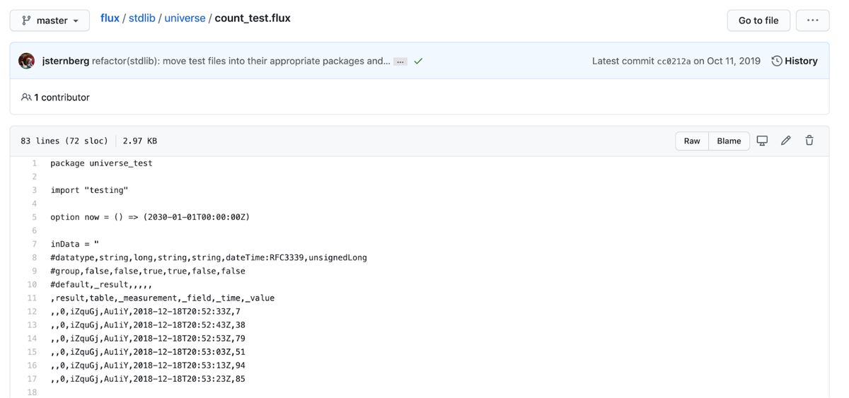<figcaption> An example of a Flux test in the universe directory in the Flux repository complete with Annotated CSV.</figcaption>

This resource is so valuable because it allows you to have a deep understanding of how Flux transforms Annotated CSV. Copy the Annotated CSV from the tests and write it to your InfluxDB instance using the csv.from() function to try out functions for yourself.

Hurdle 3: Data layout design leads to runaway cardinality and slow Flux queries

Series cardinality is the number of unique measurements, tag set, field key combinations in a bucket. Minimizing series cardinality is important for increasing query performance and decreasing your InfluxDB instance. The fastest way to avoid runaway cardinality, or rapidly growing cardinality, is to make sure that your initial schema design is good. Solution 3 will lead you through an overview of how to design a good schema.

Solution 3: Keeping general data layout recommendations in mind

To learn about data layout recommendations in detail, refer to Data Layout and Schema Design Best Practices. In general, it’s a good idea to abide by the following guidelines:

• Encode metadata in tags. Measurements and tags are indexed while field values are not. Commonly queried metadata should be stored in tags.
• Limit the number of series or try to reduce series cardinality.
• Keep bucket and measurement names short and simple.
• Avoid encoding data in measurement names.
• Separate data into buckets when you need to assign different retention policies to that data or require an authentication token.

Following these guidelines will help you control your cardinality and improve your Flux query performance. Additionally, if you can, try to anticipate common queries and let that consideration influence your schema design. If you know you’re going to frequently be querying a large subsection of data, you might want to assign a tag to that data.

To learn about ways to solve runaway cardinality with Flux in detail, refer to Monitoring Tasks and Finding the Source of Runaway Cardinality and Solving Runaway Series Cardinality When Using InfluxDB.

As an aside, if you’re interested in learning about why cardinality won’t be a point of concern for future InfluxDB users, I encourage you to read Announcing InfluxDB IOx – The Future Core of InfluxDB Built with Rust and Arrow and watch the first InfluxDB IOx Tech Talks video.

Hurdle 4: Storing the wrong data in InfluxDB and underutilizing Source Functions

Hurdle 3 is related to Hurdle 4. One of the best ways to manage your series cardinality is to make sure that you’re storing the right type of data in InfluxDB. Imagine you’re using InfluxDB to write sensor data for an Industrial IoT use case. Perhaps you’re using InfluxDB for predictive maintenance. You forecast that a particular flow gauge needs to be replaced. You have a lot of additional information about your gauge including purchase date, purchase ID, manufacturer, warranty information, item ID, etc. Some users might be inclined to include that data as a tag and write it to InfluxDB – don’t.

Solution 4: Using Source functions to pull relevant data into InfluxDB as needed

Rather than including that type of descriptive data as tags and redundantly writing this data with each flow rate measurement into InfluxDB, this relational data should be stored in the RDBMS of your choosing. Use the source functions to pull in relevant data into your InfluxDB instance ad hoc – like pulling in the item ID of a flow gauge after forecasting the need to replace it, for example. InfluxDB allows you to pull in data from a variety of sources like PostgreSQL, MySQL, Snowflake, SQLite, SQL Server, Athena and BigQuery.

Hurdle 5: Confused about how to sum across fields and project multiple aggregations

This hurdle is closely related to Hurdle 1 and Hurdle 2. You need to use the InfluxDB UI to visualize multiple aggregations, and you need to understand Annotated CSV well in order to group your data correctly to sum across fields.

Solution 5: Using the UI to project multiple aggregations and  summing across fields

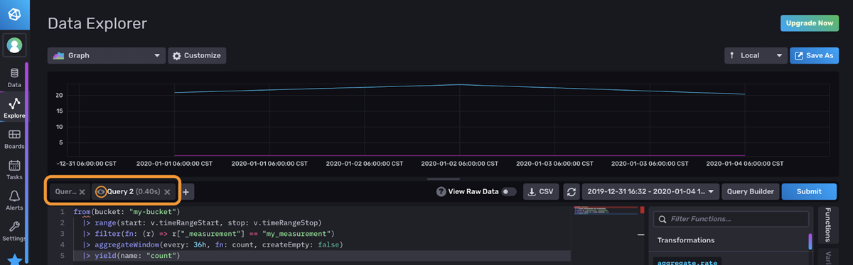
You have several options when it comes to projecting multiple aggregations with InfluxDB. The simplest is to use the UI to create multiple tabs for each aggregation. Imagine that we want to visualize both the count and the mean of a particular field. Each tab would contain a query for the mean and count, respectively.

Let’s take this multiple aggregation projection hurdle one step further by summing fields together first. Imagine that we have 4 fields:

• Electricity Supplied, ES1
• Electricity Supplied ES2
• Electricity Delivered, ED1
• Electricity Delivered, ED2

We want to visualize two series simultaneously: the Total Electricity Supplied (EST) and the Total Electricity Delivered (EDT) where EST and EDT is the sum of ES1 + ES2 and ED1 + ED2, respectively. We’ll use two tabs to visualize EST and EDT simultaneously. To sum two fields, we’ll perform the following Flux query in one query tab:

from(bucket: "p1")
  |> range(start: -24h)
  |> filter(fn: (r) => r["_measurement"] == "MyMeasurement")
  |> filter(fn: (r) => r["_field"] == "ED1" or r["_field"] == "ED2")
//group by time to isolate the values you want to sum together
  |> group(columns: ["_time"], mode:"by")
  |> sum(column: "_value")
//to ungroup your data provide a group without any columns
  |> group()
  |> yield(name: "delivered")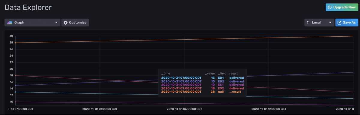

<figcaption> A Graph visualization of our data before any Flux is applied to it</figcaption>

First, we filter for two fields within one tab. The Raw Data View reveals that our data is separated into separate tables by field.

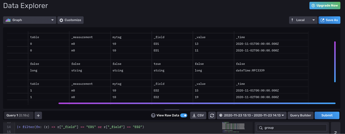<figcaption> Raw Data View of our energy data after the filter is applied</figcaption>

We have to group our data by time first so that when we apply the sum() function, we sum the fields together on that single timestamp. Notice how now the two fields, “ED1” and “ED2”, are together in the same table. Tables share the same timestamp.

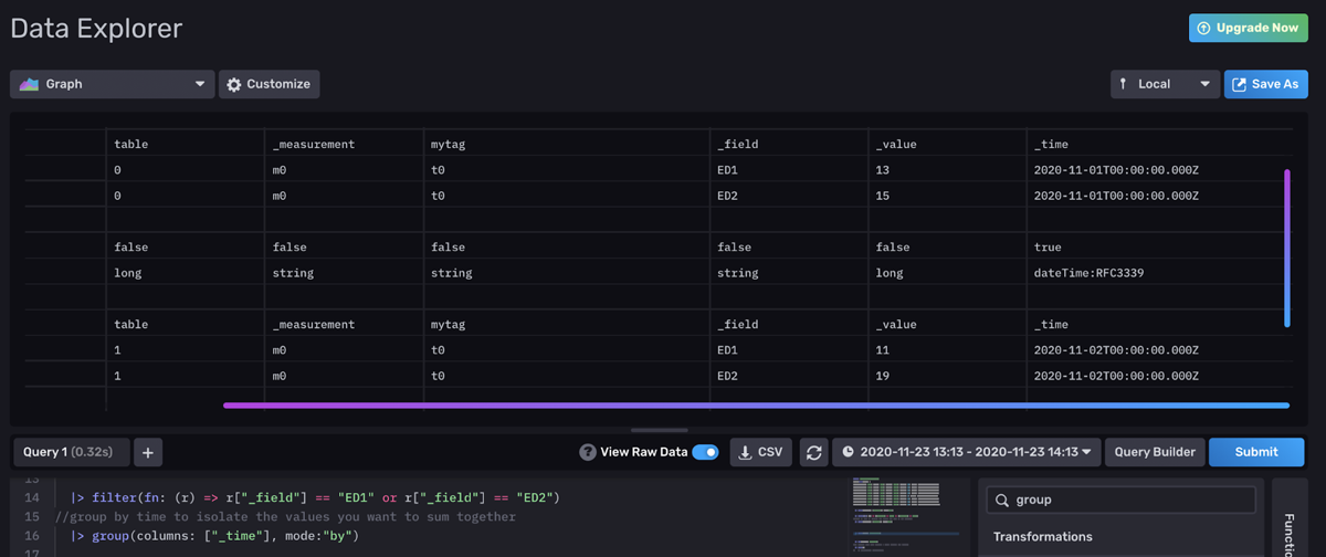<figcaption> Raw Data View of our energy data after the filter and group by time is applied</figcaption>

This step is a little unintuitive for InfluxQL users or SQL users. A closer look at the Annotated CSV explains why grouping by time is necessary. By contrast, if we don’t group by time, then we expect to get the sum() of each field for the entire range. Applying an empty group() at the end of the query effectively ungroups our data. This will ensure that our data is contained within one table rather than multiple tables, one for each timestamp. This final ungrouping changes our visualization from multiple data points represented by multiple colors to one line represented by one color.

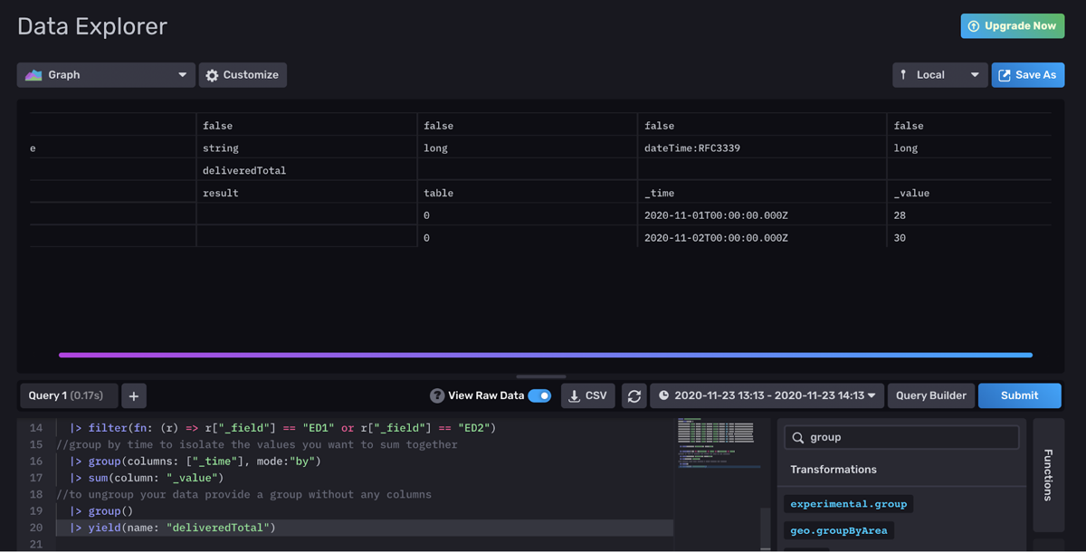<figcaption> Raw Data View of our energy data after the filter group by time, sum, and ungrouping is applied</figcaption>

Now simply open a new tab and perform a similar query with the remaining “ES1” and “ES2” fields to visualize both energy totals simultaneously.

Finally, InfluxQL and SQL users who are more accustomed to seeing fields displayed across separate columns, in one row, might find the fieldsAsCols() function useful. This function pivots your data. In fact, the entire Schema package is helpful.

You can also use Flux to restructure the data to perform multiple aggregation functions. Please refer to the “An aside: a Flux flex” section in Downsampling with InfluxDB v2.0 for information on how to use union(), join(), or reduce() to perform multiple aggregations with Flux.

Next steps for tackling Flux hurdles for Flux beginners

I hope this post helped you to tackle the Flux questions you have as a Flux beginner. If you are planning to learn Flux, please ask us for help and share your story! Share your thoughts, concerns, or questions in the comments section, on our community site, or in our Slack channel. We’d love to get your feedback and help you with any problems you run into! Your good questions are the inspiration for these posts. And once you’re ready and consider yourself an intermediate Flux user, make sure to read the next post in this series: Top 5 Hurdles for Intermediate Flux Users and Resources for Optimizing Flux.