Downsampling with InfluxDB v2.0

By Anais Dotis-Georgiou / Product, Use Cases, Developer
Oct 23, 2020

(Update: InfluxDB 3.0 moved away from Flux and a built-in task engine. Users looking to migrate from 2.x to 3.0 can use external tools, like Python-based Quix, to create tasks in InfluxDB 3.0.)

Downsampling is the process of aggregating high-resolution time series within windows of time and then storing the lower resolution aggregation to a new bucket. For example, imagine that you have an IoT application that monitors the temperature. Your temperature sensor might collect temperature data. This data is collected at a minute interval. It’s really only useful to you during the day. There isn’t any need to retain historical temperature data at that resolution, so you perform a downsampling task to only retain the mean temperatures at an hour precision instead. This downsampling helps to preserve the overall shape of your data without sacrificing unnecessary disk space. Downsampling also helps speed up queries over large time ranges because it reduces the amount of data that is evaluated as part of the query.

The benefits of downsampling: disk usage and query performance

Downsampling is a common time series database task and often a requirement for time series database users. Downsampling allows you to reduce the overall disk usage as you collect data over time. Downsampling can also improve query performance for InfluxDB OSS or Cloud. Finally, InfluxDB can ingest hundreds of thousands of points per second. Retaining that volume of that data doesn’t only create storage concerns but is also hard to work with. Downsampling allows you to eliminate the noise of high-precision time series which in turn allows you to analyze and derive value from your historical time series faster.

Downsampling gets an upgrade in InfluxDB 2.x – from continuous queries to downsampling tasks

As InfluxDB upgrades from 1.x to 2.x, so do the downsampling capabilities. In InfluxDB 1.x, users generally used continuous queries to implement downsampling at a relatively small scale. Continuous queries are created, maintained, and changed entirely through the Influx CLI tool. Continuous queries are also a standalone functionality, but as the amount of data you want to downsample increases, it has a negative impact on both the read and write performance of InfluxDB itself. At scale, the recommendation was to offload the work to Kapacitor.

In InfluxDB 2.x, you execute downsampling with a downsampling task. Tasks enable you to perform a wide variety of data processing jobs. All tasks, including downsampling, and queries in InfluxDB 2.x are written with one language – Flux. You can create tasks both through the CLI and also through the UI. Managing tasks through the UI in 2.x is the easiest way to perform a data processing job with InfluxDB. The ability to perform all of your data transformations with one tool and language also helps you better organize and visualize your time series pipeline. By contrast in the 1.x TICK stack, you must familiarize yourself with TICKscripts when working with Kapacitor, InfluxQL, and continuous query syntax to create the same data processing jobs.

Retention policies for different resolution data

In order to successfully create a downsampling task, you need to have a source bucket and a destination bucket, each with different retention policies.

• The source bucket is where you write your high precision data to.
• The destination bucket is where you write your aggregated data to.

The destination bucket should have a longer retention policy than the source bucket.

A complete downsampling task example

You can create a task with the API or with the UI. The easiest way to create a task is through the InfluxDB UI. Under the Tasks menu in the Navigation bar on the left, click Create Task. You can either create a new task, import a task, or import a task from an existing Template that you’ve also already imported (please read this documentation to learn how to import an existing Template).

Recommended workflow for task creation and debugging tasks

Imagine that I need to perform a downsampling task on my system data. For the purpose of demonstration, I will run the task every minute and aggregate my data at 10s intervals. The best way to start creating a task is to work within the Query Builder or Script Editor to create the aggregation that best suits your needs. I create the following aggregation:

from(bucket: "my-bucket")
|> range(start: v.timeRangeStart, stop: v.timeRangeStop)
|> filter(fn: (r) =>
(r["_measurement"] == "cpu"))
|> filter(fn: (r) =>
(r["_field"] == "usage_user"))
|> aggregateWindow(every: 10s, fn: mean, createEmpty: false)
// Use the to() function to validate that the results look correct. This is optional. 
|> to(bucket: "downsampled", org: "my-org")

We should just save a Flux script as a task from the Data Explorer. To save a query as a task from the Data Explorer click the Save As button in the top left corner. Make sure that you have already created a “downsampled” bucket so you can select it from the dropdown.

However, we see users encountering a copy-and-paste problem. We’ll describe this problem to highlight how to debug a task. Yet exporting a query as a task is the recommended workflow. Now that our query looks great, I copy and paste that query into my task. It looks like this:

option task = {name: "Downsampling CPU", every: 1m}

data = from(bucket: "my-bucket")
|> range(start: v.timeRangeStart, stop: v.timeRangeStop)
|> filter(fn: (r) =>
(r["_measurement"] == "cpu"))
|> filter(fn: (r) =>
(r["_field"] == "usage_user"))

data
|> aggregateWindow(every: 10s, fn: mean, createEmpty: false)
|> to(bucket: "downsampled", org: "my-org")

You can either manually write the task name and interval settings, or you can use the UI to specify those configuration options. Using the UI automatically generates the first line of our task. Next, I copy and paste my code from the Script Editor to the task. After saving the task, notice that the Task Status has failed.

To look at the logs, click the gear icon on the right of your task. Select View Task Run. Note that here is where you also have the option to export the task as a JSON object. This allows you to easily share tasks with others, which can be useful for debugging.

The View Task Runs button directs you to a list of all the times at which the processing engine tried to execute the task.

If you click View Logs, you can see the errors that caused the task failure. Here we see the error associated with the Task Run failure, “Error exhausting result iterator; Err: error @4:18-4:19: undefined identifier v: error @4:18-4:19: undefined identifier v”.

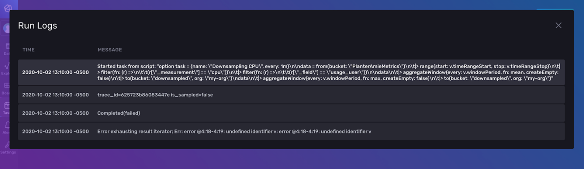
This error stems from directly copying and pasting our Flux code from the Script Editor. We need to change our time range from a variable that references the dashboard time to an actual time. Our resulting task looks like this:

option task = {name: "Downsampling CPU", every: 1m}

data = from(bucket: "my-bucket")
|> range(start: -task.every)
|> filter(fn: (r) =>
(r["_measurement"] == "cpu"))
|> filter(fn: (r) =>
(r["_field"] == "usage_user"))

data
|> aggregateWindow(every: 10s, fn: mean, createEmpty: false)
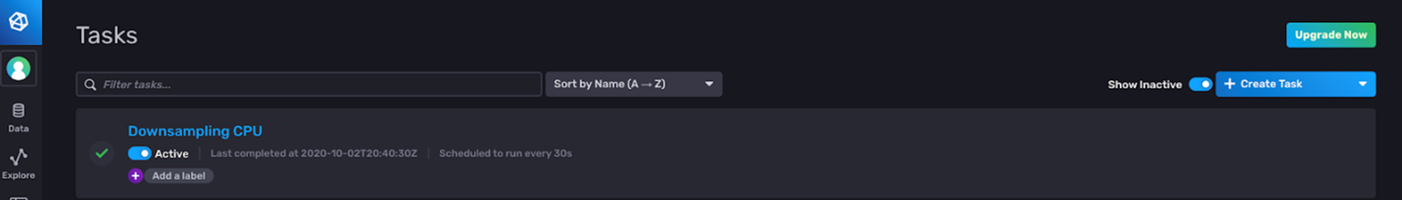
|> to(bucket: "downsampled", org: "my-org")

Now after saving the task, you can see a green arrow next to the task which indicates that it is running successfully. You can now view the data in the “downsampled” bucket.

Downsampling FAQ: multiple aggregations with Flux

Before diving into multiple aggregations with Flux, let’s address the most obvious downsampling question: “How can I get started with downsampling?”. Here is an InfluxDB template specifically for downsampling Telegraf metrics. Using this template is the easiest way to get started with downsampling.

Additionally, I’ve seen many users ask: “How can I downsample my data to retrieve the mean value and value count from my data at every aggregation interval?” This question about executing multiple aggregation projections frequently comes from InfluxDB 1.x users who are more familiar with InfluxQL than Flux. For example, they are accustomed to being able to perform the following query:

select mean(temp) as temp_mean, count(temp) as temp_count from my_measurement

And convert it into the following Continuous Query:

CREATE CONTINUOUS QUERY "cq_basic" ON "my-bucket"
BEGIN
  select mean(temp) as temp_mean, count(temp) as temp_count from my_measurement  
GROUP BY time(36h), "mytag"
END

This query and corresponding CQ would return two aggregations simultaneously. In InfluxDB 2.x, the easiest way to visualize multiple aggregations is simply to write two separate queries in multiple tabs in the UI.

For example, let’s imagine we’ve constructed a table and written the following data to InfluxDB Cloud using the array.from() and to() functions.

import "experimental/array"
array.from(rows: [{_measurement: "my_measurement", mytag: "my_tag", _field: "temp", _value: 21.0, _time: 2020-01-01T00:00:00Z,},
{_measurement: "my_measurement", mytag: "my_tag", _field: "temp", _value: 23.5, _time: 2020-01-02T00:00:00Z}, {_measurement: "my_measurement", mytag: "my_tag", _field: "temp", _value: 20.5, _time: 2020-01-03T00:00:00Z}])
|>to(bucket: "my-bucket")

Then we can query our data in two tabs.

The two queries are:

1. Mean, blue line

from(bucket: "my-bucket")
  |> range(start: v.timeRangeStart, stop: v.timeRangeStop)
  |> filter(fn: (r) => r["_measurement"] == "my_measurement")
  |> aggregateWindow(every: 36h, fn: mean, createEmpty: false)
  |> yield(name: "mean")

1. Count, pink line

from(bucket: "my-bucket")
  |> range(start: v.timeRangeStart, stop: v.timeRangeStop)
  |> filter(fn: (r) => r["_measurement"] == "my_measurement")
  |> aggregateWindow(every: 36h, fn: count, createEmpty: false)
  |> yield(name: "count")

Each query is stored within two tabs in the UI, Query 1 and Query 2. The eye icon circled in orange indicates whether or not the query from that tab is being visualized. Now that we know how to visualize multiple aggregations simultaneously, let’s learn about how to translate the CQ above into a downsampling task.

The simplest way to perform the equivalent downsampling task is to create a task per aggregation, as described in the section above. However, creating multiple tasks means querying the data multiple times. The developer should always aim to reduce workload on the query engine when creating downsampling tasks.

When a developer intends on performing multiple data transformations on top of a large subset of data, they can achieve a reduction in query engine workload by isolating the common part of the queries across all tasks. This part can then be transformed into its own task on top of which the remaining transformations will be executed. Specifically, if you’re filtering on a portion of fields or using regex for filtering, you definitely want to perform that costly query with a top-level task to avoid duplicate query work for each subsequent aggregation. Efficient task creation is also closely related to data layout and schema design.

However, the construction of a good downsampling task doesn’t end with query engine optimization considerations. Not only must the developer consider how to most efficiently write a multitude of tasks, but they must also ensure resulting data is constructed for efficient consumption.

• For example, you might want to take advantage of the set() function to add a tag to your data in the downsampling task. This way you can write your data to the same bucket and measurement. This enables the user to easily query the downsampled data.
• For example, you might append the first downsampling task to include a tag that specifies the aggregation type of your downsampling task. Now the user can easily compare downsampled data by filtering for the "agg_type" tag key.

option task = {name: "Downsampling CPU", every: 1m}

data = from(bucket: "my-bucket")
|> range(start: -2h)
|> filter(fn: (r) =>
(r["_measurement"] == "cpu"))
|> filter(fn: (r) =>
(r["_field"] == "usage_user"))

data
|> aggregateWindow(every: 10s, fn: mean, createEmpty: false)
|> set(key: "agg_type",value: "mean_cpu")
|> to(bucket: "downsampled", org: "my-org", tagColumns: ["agg_type"])

Finally, we’re ready to write a Flux translation of our CQ. The following Flux task most closely resembles the CQ above:

option task = {name: "Downsampling CPU", every: 1m}

data = from(bucket: "my-bucket")
|> range(start: -task.every)
|> filter(fn: (r) => r._measurement == "my_measurement")

data
|> mean()
|> set(key: "agg_type",value: "mean_temp")
|> to(bucket: "downsampled", org: "my-org", tagColumns: ["agg_type"])

data
|> count()
|> set(key: "agg_type",value: "count_temp")
|> to(bucket: "downsampled", org: "my-org", tagColumns: ["agg_type"])

In this example, we haven’t split the initial filtering into a separate task because we’re querying for one measurement and one field, “temp”. Since the top-level query returns data identical to our bucket’s data, creating a task that writes this filtering to a new bucket would be redundant and wasteful. However, now we can perform both aggregations within the same task. We have also changed the aggregation functions from aggregateWindow() to mean() and count(). Performing the aggregations with mean() and count() allows us to query and aggregate over shorter periods or smaller datasets, thereby increasing query efficiency. Additionally, another tradeoff to short task execution intervals is that downsampled data will be more up to date. A disadvantage of short task execution intervals is that they are less robust to data that arrives late.

An aside: a Flux flex

Flux is a powerful query language. You can take advantage of Flux to write more sophisticated queries to perform the aggregations simultaneously as well. While the downsampling approaches above are likely to be more efficient (it really depends on your schema), it’s valuable to be aware that you have multiple options when it comes to aggregating your data.

1. You can perform a union:

data = from(bucket: "my-bucket")
|> range(start: 2019-12-31T00:00:00Z, stop: 2020-01-04T00:00:00Z)
|> filter(fn: (r) => r._measurement == "my_measurement")
|> filter(fn: (r) => r._field == "temp")

temp_mean = data
|> mean()
|> set(key: "agg_type", value: "mean")
temp_count = data
|>  count()
|> toFloat()
|> set(key: "agg_type", value: "count")

union(tables: [temp_mean, temp_count])
|> group(columns: ["agg_type"], mode:"by")
|> yield()

This Flux query allows you to visualize both of your aggregations simultaneously because each aggregation is in its own “_value” column in a separate table. Here is the output in the Graph view:

Here is the output in the Table view:

1. You can either perform a join:

data = from(bucket: "my-bucket")  
  |> range(start: v.timeRangeStart, stop: v.timeRangeStop)
  |> filter(fn: (r) => r._measurement == "my_measurement")
  |> filter(fn: (r) => r._field== "temp")

 mean = data   |> aggregateWindow(every: 36h, fn: mean, createEmpty: false)

 count = data  |> aggregateWindow(every: 36h, fn: count, createEmpty: false)

join(tables: {mean: mean, count: count}, on: ["_time", "_field", "_measurement", "_start", "_stop"], method: "inner")

1. Or you can use the reduce() function to create custom aggregations. Using the reduce() function can be tricky at first though. To learn about tricks for using the reduce() function, see this blog. The following Flux script uses the reduce() function to perform both aggregations for you simultaneously:

from(bucket: "my-bucket")
|> range(start: v.timeRangeStart, stop: v.timeRangeStop)
|> filter(fn: (r) => r._measurement == "my_measurement")
|> filter(fn: (r) => r._field == "temp")
|> reduce(
fn: (r, accumulator) => ({
count: accumulator.count + 1,
sum: r._value + accumulator.sum,
mean: (accumulator.sum + r._value)/(float(v: accumulator.count + 1))
}), identity: {sum:0.0, count:0, mean:0.0 })
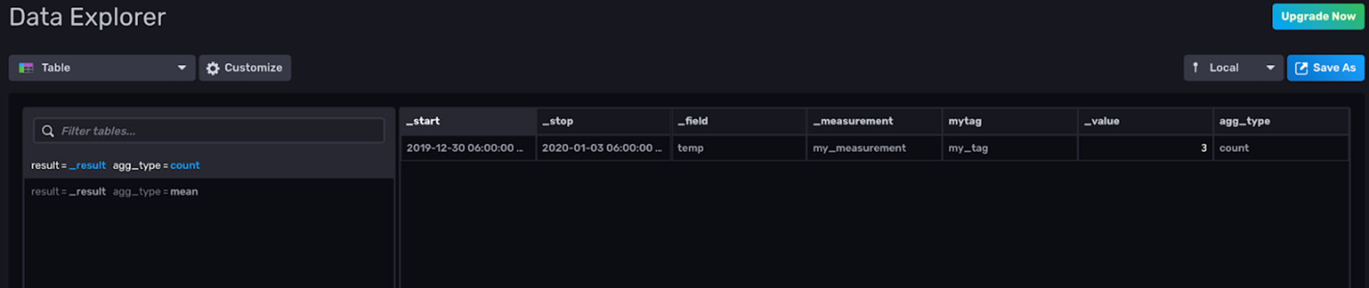
|> drop(columns: ["sum"])

Flux scripts no. 2 and 3 (above) create two columns with both of the aggregations in one table. You can’t immediately visualize the two outputs. You can use the Customize menu to select which column you want to visualize. Here we’re visualizing the count in the Graph view:

The image below is the output in the Table view. You can see that two columns, “count” and “mean”, are created and they’re in the same table.

Choosing the right query for you largely depends on your schema. The query tabs in the UI contain query run times which can help you pick the best query for your schema.

Resources for continuous query translations

I hope this InfluxDB Tech Tips blog post inspires you to take advantage of downsampling tasks with InfluxDB 2.x. If you decide to upgrade from 1.x to 2.x and need help translating your continuous queries into tasks, please ask us for help! Share your thoughts, concerns, or questions in the comments section, on our community site, or in our Slack channel. We’d love to get your feedback and help you with any problems you run into!