Why Use K-Means for Time Series Data? (Part Three)

By Anais Dotis-Georgiou / Product, Use Cases, Developer
Nov 16, 2018

In Part One of this series, I give an overview of how to use different statistical functions and K-Means Clustering for anomaly detection for time series data. In Part Two, I share some code showing how to apply K-means to time series data as well as some drawbacks of  K-means. In this post, I will share:

1. How I used K-Means and InfluxDB to detect anomalies in EKG data with the InfluxDB Python Client Library
2. How I used Chronograf to alert on the anomalies

You can find the code and the datasets I used in this repo. I am borrowing code from Amid Fish’s tutorial. It’s pretty great, and I recommend checking it out.

How I Used K-Means and InfluxDB to Detect Anomalies in EKG Data with the InfluxDB Python Client Library

If you read Part Two, then you know these are the steps I used for anomaly detection with K-means:

1. Segmentation – the process of splitting your time series data into small segments with a horizontal translation.
2. Windowing – the action of multiplying your segmented data by a windowing function to truncate the dataset before and after the window. The term windowing gets its name from its functionality: it allows you to only see the data in the window range since everything before and after (or outside the window) is multiplied by zero. Windowing allows you to seamlessly stitch your reconstructed data together.
3. Clustering – the task of grouping similar windowed segments and finding the centroids in the clusters. A centroid is at the center of a cluster. Mathematically, it is defined by the arithmetic mean position of all the points in the cluster.
4. Reconstruction – the process of rebuilding your time series data. Essentially, you are matching your normal time series data to the closest centroid (the predicted centroid) and stitching those centroids together to produce the reconstructed data.
5. Normal Error – The purpose of the Reconstruction is to calculate the normal error associated with the output of your time series prediction.
6. Anomaly Detection – Since you know what the normal error for reconstruction is, you can now use it as a threshold for anomaly detection. Any reconstruction error above that normal error can be considered an anomaly.

In the previous post, I shared how I performed Segmentation, Windowing, and Clustering to create the Reconstruction. For this post, I will focus on how I used the Python CL to perform the anomaly detection. However, before we dive into anomaly detection, let’s take a second to do some data exploration. First I use the CL to query my normal EKG data and convert it into a DataFrame.

client = InfluxDBClient(host='localhost', port=8086)
norm = client.query('SELECT "signal_value" FROM "norm_ekg"."autogen"."EKG" limit 8192')
norm_points = [p for p in norm.get_points()]
norm_df = pd.DataFrame(norm_points)
norm_df.head()

Next, I drop the timestamps and convert the “signal_value” into an array. Remember that using K-Means for anomaly detection for time series data is only viable if the time series data is regular (i.e. the interval between ti and ti+1 will always be the same). This is why I can exclude the timestamps for any of the following analysis.

ekg_data = np.array(norm_df["signal_value"])

Before we move on to Segmentation, we need to plot our normal EKG data and do some data exploration:

n_samples_to_plot = 300
plt.plot(ekg_data[0:n_samples_to_plot])
plt.xlabel("Sample number")
plt.ylabel("Signal value")
plt.show()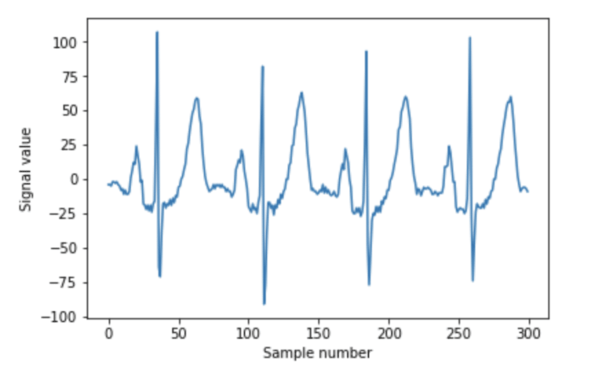

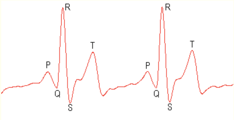
To perform segmentation, you must first decide how long you want your segments to be. If you look at the data, you can see three repeated shapes. Around “Sample number” 30, 110, 180, and 260 we see a steep peak, known as the QRX complex. Before each QRX complex, there’s a small hump. This is referred to as the P-wave. Immediately following the QRX complex, we have the T wave. It’s the second tallest peak with the largest period. We want to make sure that our segment length is long enough to encapsulate each one of those waves. Since the T wave has the longest period, we will set that period equal to the segment length where seqment_len= 32.

The EKG data is then segmented using this segmentation function:

def sliding_chunker(data, window_len, slide_len):
    """ Segmentation """
    chunks = []
    for pos in range(0, len(data), slide_len):
        chunk = np.copy(data[int(pos):int(pos+window_len)])
        if len(chunk) != window_len:
            continue
        chunks.append(chunk)

    return chunks

I store the segments in a list of arrays called test_segments:

slide_len = int(segment_len/2)
test_segments = sliding_chunker(
    ekg_data,
    window_len=segment_len,
    slide_len=slide_len
)
len(test_segments)

Next, we perform the reconstruction as described in the previous post and determine that the maximum reconstruction error for the normal EKG data is 8.8.

reconstruction = np.zeros(len(ekg_data))
slide_len = segment_len/2

for segment_n, segment in enumerate(test_segments):
    # don't modify the data in segments
    segment = np.copy(segment)
    segment = segment * window
    nearest_centroid_idx = clusterer.predict(segment.reshape(1,-1))[0]
    centroids = clusterer.cluster_centers_
    nearest_centroid = np.copy(centroids[nearest_centroid_idx])

    # overlay our reconstructed segments with an overlap of half a segment
    pos = segment_n * slide_len
    reconstruction[int(pos):int(pos+segment_len)] += nearest_centroid

n_plot_samples = 300

error = reconstruction[0:n_plot_samples] - ekg_data[0:n_plot_samples]
error_98th_percentile = np.percentile(error, 98)
print("Maximum reconstruction error was %.1f" % error.max())
print("98th percentile of reconstruction error was %.1f" % error_98th_percentile)

plt.plot(ekg_data[0:n_plot_samples], label="Original EKG")
plt.plot(reconstruction[0:n_plot_samples], label="Reconstructed EKG")
plt.plot(error[0:n_plot_samples], label="Reconstruction Error")
plt.legend()
plt.show()

Now I am ready to start the anomaly detection. First, I query my anomaly data with the Python client. Although the data is historical, this script is meant to emulate live anomaly detection. I query the data in 32-second intervals as if I were gathering it from a data stream. Next, I create the reconstruction as before and calculate the max reconstruction error for each segment. Finally, I write these errors to a new database called “error_ekg”.

while True: 
    end = start + timedelta(seconds=window_time)
    query = 'SELECT "signal_value" FROM "anomaly_ekg"."autogen"."EKG" WHERE time > \'' + str(start) + '\' and time < \'' + str(end) + '\'' 
    client = InfluxDBClient(host='localhost', port=8086)
    anomaly_stream = client.query(query)
    anomaly_pnts = [p for p in anomaly_stream.get_points()]
    df_anomaly = pd.DataFrame(anomaly_pnts)
    anomalous = np.array(df_anomaly["signal_value"])

    windowed_segment = anomalous * window
    nearest_centroid_idx = clusterer.predict(windowed_segment.reshape(1,-1))[0]
    nearest_centroid = np.copy(centroids[nearest_centroid_idx])

    error = nearest_centroid[0:n_plot_samples] - windowed_segment[0:n_plot_samples]
    max_error = error.max()

    write_time =  start + timedelta(seconds=slide_time)
    client.switch_database("error_ekg")
    json_body = [
        {
            "measurement": "ERROR",
            "tags": {
                "error": "max_error",
            },
            "time": write_time,
            "fields": {
                "max_error": max_error
            }
        }]
    client.write_points(json_body)
    print("QUERY:" + query)
    print("MAX ERROR:" + str(max_error))
    start = start + timedelta(seconds=slide_time) 
    time.sleep(32)

I get this output:

Now that I can write the max errors to a database, I am ready to use Kapacitor to set a threshold and alert on any errors that exceed my normal max reconstruction error of 8.8.

How I Used Chronograf to Alert on the Anomalies

In order to use Kapacitor, InfluxData’s data processing framework, I need to write a TICKscript, the DSL for Kapacitor, to alert on anomalies. Since I am a new Kapacitor user, I chose to use Chronograf to help me manage my alerts and autogenerate a TICKscript for me. Lucky me!

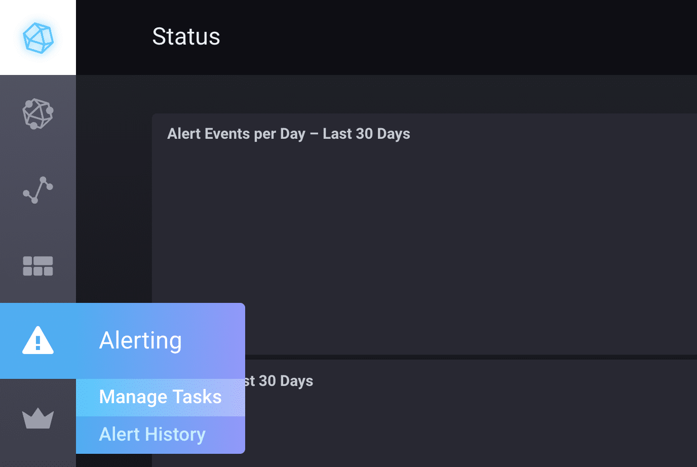
First, I navigate to the Manage Tasks page…

Next, select “Build Alert Rule”…

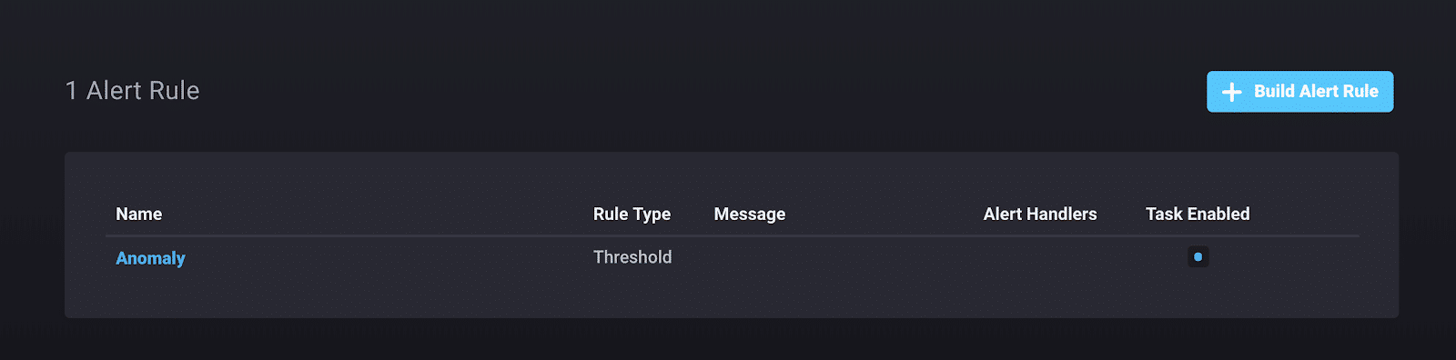
Now I can start building my alert rule. I name my alert, select the alert type…

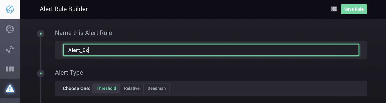
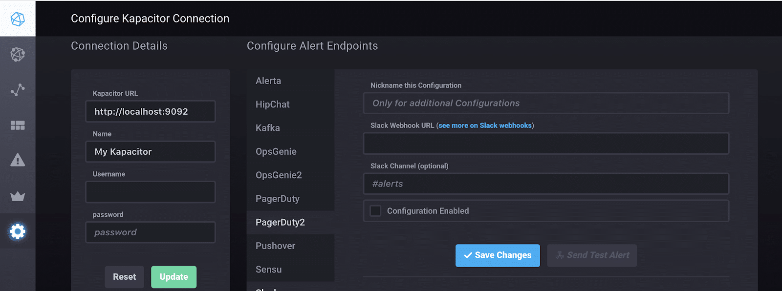
…and select the field value I want to alert on and the condition for the threshold. Finally, I specify where I want to send these alerts to…

…and configure the connection.

If I go back to the “Manage Tasks” page, I can now view the autogenerated TICKscripts. By default Kapacitor writes these alerts to the “chronograf” database. If I want to change the output database, I can simply change line 25.

var outputDB = 'chronograf'

And that’s all! As I run the while loop and send errors to the database, Kapacitor will slack me everytime my error is greater than 8.8.

If we take a look at my dashboard, you can see that I have an error greater than 8.8 at the segment that contains the anomaly and Kapacitor was able to detect it.

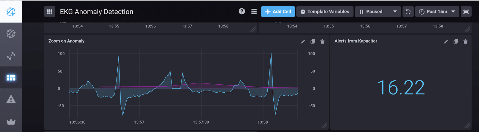
Left Cell: The magenta line represents the max reconstruction error for every 32 points. It begins to exceed 8.8 at the anomaly which occurs around 13:57:20.

Right Cell: I am displaying the max error for the anomaly with the query “SELECT max(“value”) AS “max_value” FROM “chronograf”.”autogen”.”alerts” limit 1

I hope this and the previous blog post help you on your anomaly detection journey. Please let me know if you found anything confusing or feel free to ask me for help. You can go to the InfluxData community site or tweet us @InfluxDB.

Finally, for the sake of consistency, I would like to end this blog too with a brain break. Here are some chameleons for you.