Why Use K-Means for Time Series Data? (Part Two)

By Anais Dotis-Georgiou / Use Cases, Developer
Oct 02, 2018

In “Why use K-Means for Time Series Data? (Part One)”, I give an overview of how to use different statistical functions and K-Means Clustering for anomaly detection for time series data. I recommend checking that out if you’re unfamiliar with either. In this post I will share:

1. Some code showing how K-Means is used
2. Why you shouldn't use K-Means for contextual time series anomaly detection

Some Code Showing How It's Used

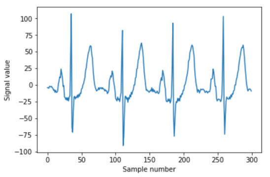
I am borrowing the code and dataset for this portion from Amid Fish’s tutorial. Please take a look at it, it’s pretty awesome. In this example, I will show you how you can detect anomalies in EKG data via contextual anomaly detection with K-Means Clustering. A break in rhythmic EKG data is a type of collective anomaly but it will we analyze the anomaly with respect to the shape (or context) of the data.

Recipe for Anomaly Detection in EKG Data using K-Means

1. Window your data

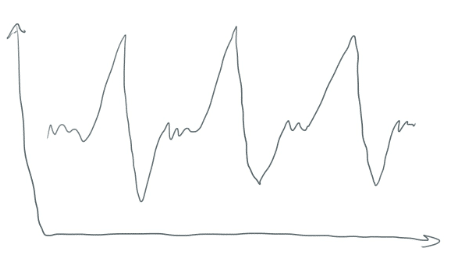
K-Means will make clusters. But how? Time series data doesn’t look like a beautiful scatter plot that is “clusterable”. Windowing your data takes data that looks like this…

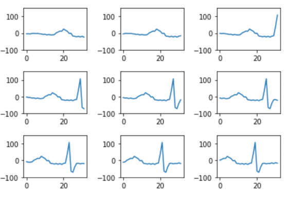
And turns it into a bunch of smaller segments (each with 32 points). They are essentially horizontal translations of each other. They look like this…

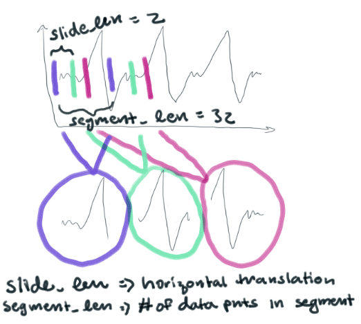
We will then take each point in each segment and graph it in a 32-dimensional space. I like to think of anything above 3-dimensions as being a nebulous cloud. You can imagine that we’re now graphing a bunch of 32-dimensional clouds in a larger space. K-Means will cluster those 32-dimensional clouds into groups based on how similar they are to each other. In this way, a cluster will represent different shapes that the data takes.

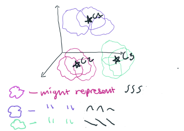
One cluster might represent a really specific polynomial function. Clusters could also represent a simple polynomial like y=x^3. The type of lines that each cluster represents is determined by your segment size. The smaller your segment size, the more you will break down your time series data into component pieces—simple polynomials. By setting our segment_len to 32 we will be making a lot of complicated polynomials.  To some extent, the number of clusters that we choose to make will determine how much we want specific coefficients of the polynomials to matter. If we make a small number of clusters, the coefficients won’t matter as much.

Here is the code for windowing your data that looks like this:

import numpy as np

segment_len = 32
slide_len = 2

segments = []
for start_pos in range(0, len(ekg_data), slide_len):
    end_pos = start_pos + segment_len
     segment = np.copy(ekg_data[start_pos:end_pos])
    # if we're at the end and we've got a truncated segment, drop it
    if len(segment) != segment_len:
        continue
    segments.append(segment)

Our segments will look like this:

We need to normalize our windows though. Later when we try to predict what class our new data belongs to, we want our output to be a continuous line. If the clusters are defined by windowed segments that do not begin with 0 and end with 0, they won’t match up when we try to reconstruct our predicted data. To do this, we multiply all of the windowed segments by a window function. We take each point in the array and multiply it by each point in an array that represents this window function:

window_rads = np.linspace(0, np.pi, segment_len)
window = np.sin(window_rads)**2
windowed_segments = []
for segment in segments:
    windowed_segment = np.copy(segment) * window
    windowed_segments.append(windowed_segment)

Now all of our segments will begin and end with a value of 0.

2. Time to Cluster

from sklearn.cluster import KMeans

clusterer = KMeans(n_clusters=150)
clusterer.fit(windowed_segments)

The centroids of our clusters are available from clusterer.cluster_centers_. They have a shape of (150,32). This is because each center is actually an array of 32 points and we have created 150 clusters.

3. Reconstruction Time

First, we make an array of 0’s that is as long as our anomalous dataset. (We have taken our ekg_data and created an anomaly by inserting some 0’s ekg_data_anomalous[210:215] = 0). We will eventually replace the 0’s in our reconstruction array with the predicted centroids.

#placeholder reconstruction array

reconstruction = np.zeros(len(ekg_data_anomalous))

Next, we need to split our anomalous dataset into overlapping segments. We will make predictions based on these segments.

slide_len = segment_len/2
# slide_len = 16 as opposed to a slide_len = 2. Slide_len = 2 was used to create a lot of horizontal translations to provide K-Means with a lot of data. 

#segments were created from the ekg_data_anomalous dataset from the code above
for segment_n, segment in enumerate(segments):
    # normalize by multiplying our window function to each segment
    segment *= window
    # sklearn uses the euclidean square distance to predict the centroid
    nearest_centroid_idx = clusterer.predict(segment.reshape(1,-1))[0]
    centroids = clusterer.cluster_centers_
    nearest_centroid = np.copy(centroids[nearest_centroid_idx])

    # reconstructed our segments with an overlap equal to the slide_len so the centroids are       
    stitched together perfectly. 
    pos = segment_n * slide_len
    reconstruction[int(pos):int(pos+segment_len)] += nearest_centroid

Finally, determine whether we have greater than a 2% error and plot.

error = reconstruction[0:n_plot_samples] - ekg_data_anomalous[0:n_plot_samples]
error_98th_percentile = np.percentile(error, 98)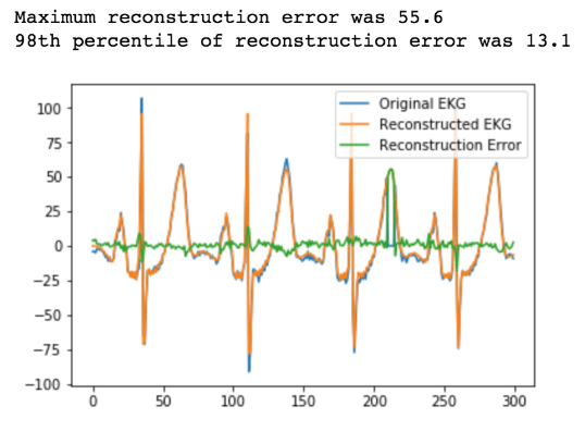

4. Alerting

Now if we wanted to alert on our anomaly, all we have to do is set a threshold of 13.1 for our Reconstruction Error. Anytime it exceeds 13.1, we have detected an anomaly.

Now that we’ve spent all this time learning and understanding K-Means and its application in contextual anomaly detection, let’s discuss why it could be a bad idea to use it. To help you get through this part, I will offer you this brief brain break:

Why You Shouldn't Use K-Means for Contextual Time Series Anomaly Detection

I learned a lot about the drawbacks of using K-Means from this post. That post goes into a lot of detail, but three major drawbacks include:

1. K-Means only converges on the local minima to find centroids.

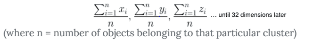
When K-Means finds centroids, it first plots 150 random “points” (in our case it’s actually a 32-dimensional object, but let’s just reduce this problem to a 2-dimensional analogy for a second). It uses this equation to calculate the distance between all 150 centroids and every other “point”. Then it takes a look at all those distances and groups the objects together based on their distance. Sklearn calculates the distance with the Squared Euclidean Difference (this is faster than using just the Euclidean difference). It then updates the centroid’s position based on this equation (you can think of it kinda like the average distance from the objects in a cluster).

Once it cannot be updated anymore, it determines that that point is the centroid. However, K-Means can’t really “see the forest through the trees”. If the initial randomly placed centroids are in a bad location, then K-Means won’t assign a proper centroid. Instead, it will converge on a local minimum and provide poor clustering. With poor clustering comes poor predictions.  To learn more about how K-Means finds centroids, I recommend reading this. Look here to learn more about how K-Means converges on local minima.

1. Each timestep is cast as a dimension.

Doing this is fine if our time-steps are uniform. However, imagine if we were to use K-Means on sensor data. Assume your sensor data is coming in at irregular intervals. K-Means could really easily produce clusters that are prototypical of your underlying time series behavior.

1. Using the Euclidean distance as a similarity measure can be misleading.

Just because an object is close to a centroid doesn’t necessarily mean that it should belong to that cluster. If you took a look around, you might notice that every other nearby object belongs to a different class. Instead, you might consider applying KNN using the objects in the clusters created by K-Means.

I hope this and the previous blog help you on your anomaly detection journey. Please let me know if you found anything confusing or feel free to ask me for help. You can go to the InfluxData community site or tweet us @InfluxDB.