Data Layout and Schema Design Best Practices for InfluxDB
By
Anais Dotis-Georgiou
updated December 14, 2025
Product
Use Cases
Developer
Navigate to:
Figuring out the best data layout for InfluxDB v2 is important in optimizing the resources used by InfluxDB, as well as improving ingestion rates and the performance of queries and tasks. You also want to consider developer and user experience (UX). This post will walk you through developing a schema for an IoT application example and answer the following questions:
- What are general recommendations for schema design and data layout for InfluxDB v2?
- What impacts computing resources such as memory, CPU, and storage? How do I optimize InfluxDB for the available resources?
- What is series cardinality?
- How do I calculate series cardinality?
- How are series cardinality and ingest rate related?
- What is downsampling? When should I perform downsampling?
- How do I reduce my resource usage?
- How do I optimize my InfluxDB schema for increased query and downsampling performance?
- What other considerations should I take when designing my InfluxDB schema?
- How will my organization interact with the data? How does UX design affect schema?
- How do security and authorization considerations impact my schema design?
- What are some common schema design mistakes?
TL;DR General recommendations for schema design and data layout
Generally, you should abide by the following recommendations:
- Encode meta data in tags. Measurements and tags are indexed while field values are not. indexed. Commonly queried metadata should be stored in tags. Tags values are strings, while fields values can be strings, floats, integers, or booleans.
- Limit the number of series or try to reduce series cardinality.
- Keep bucket and measurement names short and simple.
- Avoid encoding data in measurement names.
- Separate data into buckets when you need to assign different retention policies to that data or require an authentication token.
Minimizing your InfluxDB instance
This section introduces InfluxDB concepts that impact the resources required to run your InfluxDB instance. We’ll learn about:
- Series cardinality
- How to calculate series cardinality
- How ingest rate affects InfluxDB instance size
- Downsampling
Series cardinality
You should aim to reduce series cardinality in an effort to minimize your InfluxDB instance size and costs. Series cardinality is the number of unique bucket, measurements, tag sets, and field keys combinations in an organization. InfluxDB uses a time series index called TSI. TSI enables InfluxDB to handle extremely high series cardinality. TSI supports high ingest rates by pulling commonly queried data in memory and moving infrequently accessed data on disk. Designing your data schema to reduce series cardinality requires some foresight and planning.
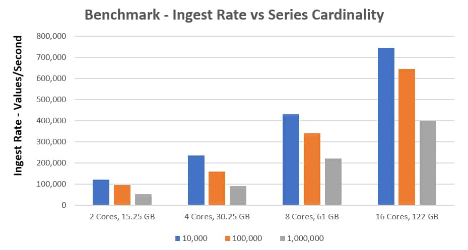
In the above graph, the blue, orange, and grey lines represent different series cardinalities. For example, if you’re running InfluxDB on a r4.4xl instance with a series cardinality of 10,000 you can ingest over 700,000 points per second.
Calculate cardinality
Before we think about how to optimize our data schema to reduce series cardinality. Let’s calculate the series cardinality for a plant monitoring app, MyPlantFriend. MyPlantFriend monitors a user’s plants’ environment (storing temperature, humidity, moisture, and light metrics). The data layout looks like this:
| Bucket | MyPlantFriend |
| Measurement | MyPlantFriend |
| Tag Keys |
|
| Field Keys |
|
Let’s assume that we have two users and several types of plant_species:
| user | plant _species |
| cool_plant_lady | orchid |
| cool_plant_lady | common cactus |
| succulexcellent | prickly pear |
| succulexcellent | aloe vera |
| succulexcellent | jade plant |
We see we have 2 tag keys. For the user tag key, we have 2 tag values. For the plant_species tag key we have 5 tag values.
We have 1 bucket, 1 measurement, and 4 field keys.
Our series cardinality would be equal to:

Your first priority is to avoid runaway series cardinality. Runaway series cardinality happens when you load your tags or measurements with data that is potentially unbounded. The example above is a perfect example of schema that will likely lead to runaway series cardinality. Assuming your users will grow, containing the username in a tag is a quick way to have your cardinality explode. Instead, it would be prudent to keep the username as a field. Additional examples of runaway series cardinality are in the final section of this blog.
How ingest rate affects InfluxDB
Series cardinality only tells half of the dimensionality and performance story of your InfluxDB instance. Minimizing series cardinality should be a part of your strategic planning effort to minimize your costs and InfluxDB size, but you have to contextualize the series cardinality within the series ingest rate. The frequency of series ingest plays a big part in your overall instance size.
For example, imagine if I added some user metrics to the MyPlantFriend measurement, like device ids and email addresses. This information shouldn’t be written to the database everytime we write a new environment metric. Writing the same email address every time a temperature metric is written is redundant. In fact, we probably only want to write that data once, upon user registration. Therefore it makes sense to write this user data to a different bucket. However, this example is specific to the MyPlantFriend IoT application where we are assuming that fields are unrelated to each other. Please read the section “Final considerations for InfluxDB Schema design” to understand how UX affects schema design.
Writing our datasets (user data and MyPlantFriend metrics) into separate buckets provides the following advantages:
- We can write the data once upon registration and decrease the ingest volume
- Buckets are at the top level of the organizational hierarchy in the InfluxDB schema and have a retention policy associated with them–a duration of time that each data point persists. Separating data into different buckets allows us to assign different retention policies to our data. For example, the user data bucket would have an infinite retention policy. Whereas, the MyPlantFriend bucket would have a short retention policy since sensor metrics are gathered at a high frequency and retaining historical data isn't important.
- We can optimize our common queries and downsampling tasks for performance. We'll describe the relationship between instance size, schema design, and query performance in the following section.
Downsampling
Similarly to how we differentiated our data into different buckets to apply separate retention policies, we must also think about how we want to downsample our data. Downsampling is the process of using a task to aggregate your data from its high precision form into a lower precision form. For example, downsampling tasks for MyPlantFriend might look like:
- Downsampling the hourly temperature and light metrics to weekly min and max values.
- Downsampling the hourly soil moisture and humidity metrics to daily averages.
Used in combination with retention policies, downsampling allows you to reduce InfluxDB’s instance size because queries against downsampled data scan, process, and transfer less data. You should perform downsampling whenever you can afford to lose high precision data or when your queries can be exactly answered with downsampled aggregates. Employ retention policies to drop your old high precision data. This will save you on storage and increase query performance.
Optimizing your schema for resource usage
Understanding when to apply downsampling is fairly straightforward, however optimizing your InfluxDB schema to increase your downsampling task performance and reduce your resource usage isn’t trivial. Thinking more deeply about downsampling directs us towards a new schema design. Remember that buckets, measurements, and tags are indexed while field values are not. Therefore queries and tasks that filter by buckets, measurements, and tags are more performant than those that filter for fields. Since we foresee downsampling the MyPlantFriend fields (air_temp, soil_moisture, humidity, and light across) at different rates, splitting the fields across measurements offers the following advantages:
- Querying is simpler (this can be especially useful if you intend on creating templates or recycling queries across organizations).
- Example of a Flux query for 4 fields in one measurement
from(bucket: "MyPlantFriend")
  |> range(start: v.timeRangeStart, stop: v.timeRangeStop)
  |> filter(fn: (r) => r["_measurement"] == "MyPlantFriend")
  |> filter(fn: (r) => r["_field"] == "light")
|> max()- Example of a Flux query after splitting fields into separate measurements:
from(bucket: "MyPlantFriend")
  |> range(start: v.timeRangeStart, stop: v.timeRangeStop)
  |> filter(fn: (r) => r["_measurement"] == "light")
|> max()- The latter query is simpler, more performant, and reduces memory usage.
The importance of optimizing schema design for query and task performance is proportional to your task number and frequency. After verifying that you don’t have a runaway series cardinality problem, you want to strike a balance between minimizing series cardinality, reducing instance size through downsampling and retention policies, and optimizing schema design for query and task performance.
Final considerations for InfluxDB schema design
Thinking about the influence that series cardinality, data ingest rate, and query performance has on instance size is only part of a well thought out data schema design. You also want to think about how your users and developers interact with your time series data to optimize your InfluxDB schema for developer experience.
The MyPlantFriend fields aren’t really related to each other. I don’t foresee the user needing to compare fields with each other or perform math across the fields. This supports the proposition to separate the fields out into measurements. Let’s contrast the MyPlantFriend UX with the UX of a human health app to highlight how UX influences schema design. Humans have a standard set of biological health indicators. For a human health app I would write blood oxygen level, heart rate, and body temperature in one measurement because I foresee needing to compare a combination of the metrics to assess human health. While you could separate out the fields into different measurements for a human health app, you’d most likely have to use joins() to perform math across measurements or buckets which are more computationally expensive.
By contrast, separating out the fields for the MyPlantFriend app into different measurements is a good strategy because joins() will most likely not be used or used sparingly. This schema change for the MyPlantFriend will allow developers to write queries easily and provide the users with the data they’re interested in.
Additionally, if you’re creating an app and using the API, you want to address security and authorization concerns by writing data associated with each user to a separate bucket. InfluxDB authentication tokens ensure secure interaction between users and data. A token belongs to an organization and identifies InfluxDB permissions within the organization. You can scope tokens to individual buckets.
Final schema proposal
After taking runaway cardinality, downsampling and retention policies, and query performance optimization into consideration, I propose the following schema design:
| Bucket (Retention Policy = 2 Weeks) | WetMetrics |
| Measurement | airt_temp |
| Measurement | light |
| Field | air_temp |
| Field | light |
| Bucket (Retention Policy = 2 Days) | DryMetrics |
| Measurement | humidity |
| Measurement | soil_moisture |
| Field | humidity |
| Field | soil_moisture |
| Bucket (Retention Policy = Inf) | UserData |
| Measurement | user_data |
| Tag | region |
| Field | username |
| Field | plant_species |
Remember, the final schema results from taking the following assumptions specific to the MyPlantFriend IoT Application into consideration:
- The username and plant species should be converted into a field to avoid runaway series cardinality.
- Dry and wet metrics required different downsampling and retention policies, which lends them to being split into separate buckets.
- The fields are unrelated to each other and performing math across measurements and/or buckets will be very rare. If fields are related, they should be contained within the same measurement.
- A tag for region is added to provide an example for what a good tag looks like. The number of possible regions is scoped, so this won't cause runaway cardinality.
Common schema design mistakes that lead to runaway cardinality
Mistake 1: Log messages as tags. Solution 1: We don’t advise that anyone store logs as tags due to the potential for unbounded cardinality (e.g. logs likely contain unique timestamps, UUIDs, etc). You can store attributes of a log as a tag, as long as the cardinality isn’t unbounded. For example, you could extract the log level (error, info, debug) or some key fields from the log message. Storing logs as a field is ok, but it is less efficient to search (essentially table scans), compared to other solutions.
Mistake 2: Too many measurements. This typically happens when people are moving from - or think of InfluxDB as - a key-value store. So for example, if you’re writing system stats to an InfluxDB instance you might be inclined to write data like so: Cpu.server-5.us-west.usage_user value=20.0
Solution 2: Instead encode that information as tags like so: cpu, host=server-5, region = us-west, usage_user=20.0
Mistake 3: Making ids (such as eventid, orderid, or userid) a tag. This is another example that can cause unbounded cardinality if the tag values aren’t scoped. Solution 3: Instead, make these metrics a field.
I hope this tutorial helps you understand how to best design your InfluxDB schema. As always, if you run into hurdles, please share them on our community site or Slack channel. We’d love to get your feedback and help you with any problems you run into.
